5. Construction of a joint element

The crack trajectory \(\Gamma\) is defined a priory, so it can be discretized by joint elements. The sub-domains \({\Omega }^{\text{+}}\) and \({\Omega }^{\text{-}}\), located on either side of \(\Gamma\), are discretized by classical solid THM elements in such a way that their nodes at the interface coincide.

5.1. Degrees of interpolation of degrees of freedom

The joint element with hydro-mechanical coupling uses the mechanical formulation of conventional joint elements (but by changing from a linear element to a quadratic element) and interacts with the neighboring elements THM. The degrees of interpolation of the degrees of freedom is therefore chosen in coherence with these neighboring elements.

In order to be compatible with the THM elements of the massif:

• the movements are interpolated quadratically (\(\mathit{P2}\) -continuous)

• the pressures are interpolated linearly (\(\mathit{P1}\) -continuous).

A degree of freedom that does not pre-exist in either of the two previous elements appears in the formulation. This is the hydraulic Lagrange multiplier (variables \({q}^{\text{+}}\) and \({q}^{\text{-}}\) in the variational equations at). The degree of interpolation of these hydraulic Lagrange multipliers must be chosen in such a way as to respect a discrete LBB condition. They are therefore taken to be constant by element.

5.2. Item description

The constructed element has zero thickness and the entire crack path is meshed with this element. The lower and upper edges are connected to the rest of the structure. The flow of fluid along the crack is written along the middle plane of the element (in gray in the figure).

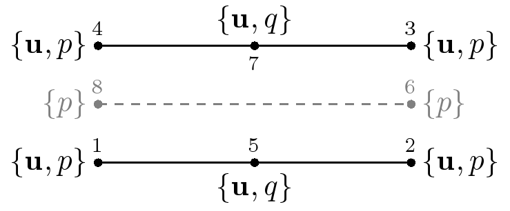
Figure 5.2.1: « Exploded » view of the joint element with hydro-mechanical coupling and without propagation