3. Introduction of field \(\theta\)

3.1. Conditions to be met

Field \(\theta\) is a vector field, defined on the cracked solid, which represents the transformation of the domain during crack propagation in the sense of [§1]. The transformation should only change the position of the crack bottom and not the edge of the \(\delta \Omega\) domain, i.e.: \(\theta \mathrm{.}n=0\) on (\(n\) normal to \(\delta \Omega\)). Also, the field \(\theta\) must be regular on \(\Omega\) [bib4].

Because of the uniqueness of the field of movement, it is interesting from a numerical point of view to use constant \(\theta\) fields in a neighborhood of \({\Gamma }_{0}\), thus cancelling out in this neighborhood the singular terms \(\psi {\theta }_{k,k}-{\sigma }_{\mathrm{ij}}{u}_{i,p}{\theta }_{p,k}\) in \(G(\theta )\).

3.2. Choice of field \(\theta\) in dimension 3

3.2.1. Construction method

We need to build a field \(\theta\) verifying:

\(\{\begin{array}{cc}{\theta }_{n}=\theta \mathrm{.}n=0& \text{sur le bord du domaine}\delta \Omega (n\text{est la normale à}\delta \Omega )\\ \stackrel{ˉ}{\theta }=\stackrel{ˉ}{{\theta }_{0}}& \text{donné sur le fond de fissure}{\Gamma }_{0}\end{array}\)

where \(\stackrel{ˉ}{\theta }\) represents the trace of \(\theta\) on \({\Gamma }_{0}\).

We give ourselves two toric surfaces \(T\) and \(S\) (deformed cylinders) surrounding the bottom of the crack \({\Gamma }_{0}\mathrm{.}\) To verify the first condition above, it is necessary in particular to ensure that the ring \(S\) is strictly included in \(\Omega\).

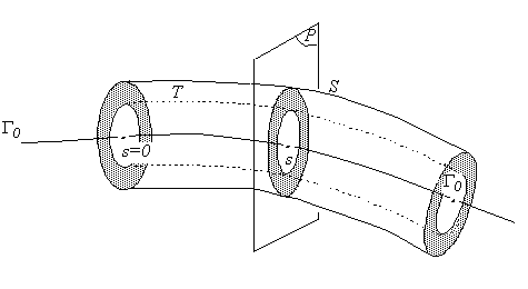
Figure 3.2.1-a: Field construction \(\theta\) in 3D (overview)

We note \({R}_{\mathrm{inf}}(s)\) the variable radius of \(T\) and \({R}_{\text{sup}}(s)\) the variable radius of \(S\).

Figure 3.2.1-b: Field construction \(\theta\) in 3D (section plane)

At any point in \({\Gamma }_{0}\), identified by its curvilinear abscissa \(s\), we can define a normal plane \(P\) in which the field \(\theta\) is introduced in the following way:

• \({\theta }_{n}(r(s))=\stackrel{ˉ}{{\theta }_{0}}(s)\text{pour}0\le r(s)\le {R}_{\mathrm{inf}}(s)\)

• \({\theta }_{n}(r(s))=0\text{pour}r(s)\ge {R}_{\text{sup}}(s)\)

• \({\theta }_{n}\) varies linearly with respect to radius \(r(s)\) in corona \(S({R}_{\text{sup}}(s))\setminus T({R}_{\mathrm{inf}}(s))\)

• \({\theta }_{n}\) is continuous in \(S({R}_{\text{sup}}(s))\).

This way of introducing \(\theta\) is geometric. It is equivalent to giving yourself two rays \({R}_{\mathrm{inf}}(s)\) and \({R}_{\text{sup}}(s)\), and to performing distance calculations from a current point to the bottom of the crack to determine the value of \(\theta\) at this point.

3.2.2. Calculation algorithms

Since the module \(\mid \theta \mid\) of field \(\theta\) is given all over the crack background \({\Gamma }_{0}\) (by the user or by the method \(\theta\), see [§2.3]), the problem is to determine the field \(\theta\) (norm and direction) at any point in the domain \(\Omega\).

We denote \({\mid \theta \mid }_{i}\), \({R}_{\mathrm{inf}i}\) and \({R}_{\text{sup i}}\) respectively \({\Gamma }_{0}\) the module of the field \(\theta\), the radii \({R}_{\mathrm{inf}}\) and \({R}_{\text{sup}}\) for the \(i\) -th node of the crack bottom.

The procedure for calculating field \(\theta\) at any point in \(\Omega\) is as follows:

• Field calculation \(\theta\) at each point of \({\Gamma }_{0}\) : given the module \({\mid \theta \mid }_{i}\), the problem is to determine the direction of \(\theta\). \(\theta\) should be locally in the tangential plane to the lips of the crack and normal to the edge to which it belongs. \(\theta\) being calculated at the nodes, in the general case (non-plane crack background) the direction of \(\theta\) will be averaged over the 2 edges of \({\Gamma }_{0}\) that have the node in common.

Figure 3.2.2-a: Field construction \(\theta\) in 3D (normal)

Let \({F}_{1}\) and \({F}_{2}\) be two faces belonging to the lips of the crack and including the successive edges \({T}_{1}\) and \({T}_{2}\) of \({\Gamma }_{0}\). First, we calculate the normal \({n}_{1}\) to the edge \({T}_{1}\) in the plane of the face \({F}_{1}\) and then the normal \({n}_{2}\) to the edge \({T}_{2}\) in the plane of the face \({F}_{2}\).

\({n}_{1}\) and \({n}_{2}\) being unit normals, we deduce \(n=\frac{{n}_{1}+{n}_{2}}{2}\) then \(\theta (M)=\mid \theta (M)\mid n\) for \(M\in {\Gamma }_{0}\).

We consider faces \({F}_{i}\) to be straight:

• In the case where \({F}_{i}\) is a triangle, the plane of the \({F}_{i}\) face is defined.

• In the case where \({F}_{i}\) is a quadrangle, we cut \({F}_{i}\) into 2 triangles \({F}_{\mathrm{i1}}\) and \({F}_{\mathrm{i2}}\). We must then calculate the equations of the two planes containing faces \({F}_{\mathrm{i1}}\) and \({F}_{\mathrm{i2}}\) and do two normal calculations per edge \({T}_{i}\).

This calculation requires knowing the faces belonging to the lips of the crack and comprising an edge of \({\Gamma }_{0}\). The user enters all the surface elements belonging to the lips of the crack. These faces appear in one or more groups of meshes and are described in the connectivities of the surface elements. The algorithm sorts these faces to keep only those with 2 vertices on \({\Gamma }_{0}\). The steps of the algorithm are as follows:

• For each node in \({\Gamma }_{0}\), the meshes belonging to the lips of the crack are extracted,

• From these stitches, we sort the ones with two knots on \({\Gamma }_{0}\),

• We get the type of the face (TRIA or QUAD) and we calculate the equation of the tangent plane (s),

• For each edge of \({\Gamma }_{0}\) of vertices \({N}_{i}\), \({N}_{i+1}\) calculate the normals \({n}_{i\mathrm{,1}}\), \({n}_{i+\mathrm{1,1}}\), \({n}_{i\mathrm{,2}}\) and \({n}_{i+\mathrm{1,2}}\).

Finally, \(\theta\) is calculated using the following algorithm:

Loop on summits \({N}_{i}\) of \({\Gamma }_{0}\): \(\begin{array}{}{n}_{i}=\frac{1}{2}({n}_{i\mathrm{,1}}+{n}_{i\mathrm{,2}})\\ \theta ({N}_{i})={\mid \theta \mid }_{i}{n}_{i}\end{array}\)

End of the loop on summits \({N}_{i}\) of \({\Gamma }_{0}\)

Figure 3.2.2-b: Notations of normals at the bottom of a crack

• Calculating the projection \({\Gamma }_{0}\) of each point of \(\Omega\):

For each \(M\) node:

• Retrieving the coordinates of \(M\)

• Loop on knots \({N}_{k}\) from \({\Gamma }_{0}\) \(k=\mathrm{1,}\mathrm{NNO}-1\)

Retrieving the coordinates of \({N}_{k}\) and \({N}_{k+1}\)

Calculation of \({s}_{k}=\frac{{N}_{k}{N}_{k+1}\mathrm{.}{N}_{k}M}{\parallel {N}_{k}{N}_{k+1}\parallel }\)

\(\begin{array}{}/{s}_{k}<0:{s}_{k}=0\\ /{s}_{k}>1:{s}_{k}=1\end{array}\)

Calculating the coordinates of \(\stackrel{ˉ}{{M}_{k}}:O\stackrel{ˉ}{{M}_{k}}=O\stackrel{ˉ}{{N}_{k}}+{s}_{k}{N}_{k}{N}_{k+1}\)

Calculation of \({d}_{k}=d(M,\stackrel{ˉ}{{M}_{k}})\)

End loop

• Retrieving \(i\) such as \({d}_{i}=\underset{k}{\mathrm{min}}({d}_{k})\)

• Knowing \(i\), we get \({N}_{i},{N}_{i+1},{s}_{i}\) and the projection \(\stackrel{ˉ}{M}\) of \(M\) on \({\Gamma }_{0}\) such as:

\({N}_{i}\stackrel{ˉ}{M}={s}_{i}{N}_{i}{N}_{i+1}\)

• Field calculation \(\theta\) at each point of \(\Omega\):

Buckle on knots \(M\)

• Calculation of the projection \(\stackrel{ˉ}{M}\) of \(M\) on \({\Gamma }_{0}\) (cf. above: gives \({N}_{i},{N}_{i+1},{s}_{i}\))

• Calculation of \(d=d(M,\stackrel{ˉ}{M})\)

• Calculation of \(\theta (\stackrel{ˉ}{M})\) by linear interpolation:

\(\theta (\stackrel{ˉ}{M})=(1-{s}_{i})\theta ({N}_{i})+{s}_{i}\theta ({N}_{i+1})\)

• Calculation of \({R}_{\mathrm{inf}}({s}_{i})\) and \({R}_{\text{sup}}({s}_{i})\) by linear interpolation:

\({R}_{\mathrm{inf}}({s}_{i})=(1-{s}_{i}){R}_{\mathrm{inf}i}+{s}_{i}{R}_{\mathrm{inf}i+1}\)

\({R}_{}({s}_{i})=(1-{s}_{i}){R}_{\text{sup i}}+{s}_{i}{R}_{\text{sup}i+1}\)

• \(\begin{array}{}/\text{Si}d>{R}_{\text{sup}}({s}_{i}),\theta (M)=0\\ /\text{Si}d<{R}_{\mathrm{inf}}({s}_{i}),\theta (M)=\theta (\stackrel{ˉ}{M})\\ /\text{Si}{R}_{\mathrm{inf}}({s}_{i})\le d\le {R}_{\text{sup}}({s}_{i}),\alpha =\frac{d-{R}_{\mathrm{inf}}({s}_{i})}{{R}_{\text{sup}}({s}_{i})-{R}_{\mathrm{inf}}({s}_{i})}\text{et}\theta (M)=(1-\alpha )\theta (\stackrel{ˉ}{M})\end{array}\)

End loop

Figure 3.2.2-d: Field calculation \(\theta\) in 3D

3.3. Choice of field \(\mathrm{\theta }\) in dimension 2

This is a particular case of dimension 3. \({\mathrm{\Gamma }}_{0}\) is limited to one point, the user chooses rays \({R}_{\mathrm{inf}}\) and \({R}_{\text{sup}}\), the module \(\theta\) at the bottom of the crack \(\mid {\theta }_{0}\mid\) and the field \(\theta\) is constructed in such a way that:

\(\begin{array}{}\theta (r)=0\text{si}r\ge {R}_{\text{sup}}\\ \theta (r)=\mid {\theta }_{0}\mid n\text{si}r\le {R}_{\mathrm{inf}}\\ \theta (r)=\frac{{R}_{\text{sup}}-r}{{R}_{\text{sup}}-{R}_{\mathrm{inf}}}\mid {\theta }_{0}\mid n\text{si}{R}_{\mathrm{inf}}\le r\le {R}_{\text{sup}}\end{array}\)

To verify condition \(\theta \mathrm{.}n=0\) on \(\delta \Omega\), it is especially necessary to ensure that the ring with radius \({R}_{\text{sup}}\) is strictly included in \(\Omega\).

^

Figure 3.3-a: Calculation of field \(\theta\) in 2D

3.4. Alternative method: field \(\theta\) defined according to the number of layers

Alternatively, the use of the operands NB_COUCHE_INF and NB_COUCHE_SUP makes it possible to define the integration crowns of the field \(\theta\) not in terms of radius, but in terms of the number of layers of elements. The concept of layer is defined here by the connectivity of the mesh: the first layer of elements consists of all the elements connected to the crack front \({\Gamma }_{0}\), the second layer of elements consists of all the elements connected to the first layer, and so on.

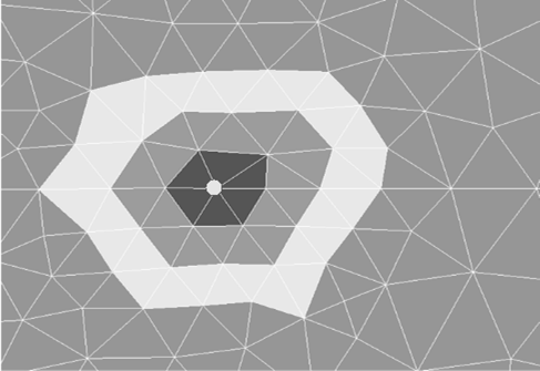
Figure 3.4: Element layers 1 to 3 around the crack front (2D)

Field \(\theta\) being a node field, we derive a notion of node layer from the concept of element layer:

• Crack front nodes are assigned the layer number 0

• The vertex nodes of the elements in the first element layer (excluding nodes in the front) are assigned the number layer 1.

• The vertex nodes of elements in the second element layer (excluding nodes in the first layer) are assigned the number layer 2.

• And so on until you reach layer number NB_COUCHE_SUP. All nodes outside the crown thus defined are assigned the layer number NB_COUCHE_SUP.

• Any middle edge nodes are assigned a layer number equal to the average of the edge’s vertex node layer numbers.

Once each node in the mesh has a layer number, field \(\theta\) is calculated using the methods described in sections 3.2 (3D) and 3.3 (2D). R_ SUP and R_ INF are then simply replaced by NB_COUCHE_SUP and NB_COUCHE_INF, and the distance from the node to the crack front is replaced by the node’s layer number.

3.5. Alternative method

The user can enter field \(\mathrm{\theta }\) himself, using the CREA_CHAMP [U4.72.04] command, using the [] command, which allows to assign \(\theta\) node by node or group of nodes.