2. Discretization of the energy return rate#
2.1. Method \(\theta\) in dimension 2#
It should be noted that the energy return rate
is the solution of the variational equation:
\(\underset{{\mathrm{\Gamma }}_{0}}{\int }G(s)\mathrm{\theta }(s)\mathrm{.}m(s)\mathit{ds}=G(\mathrm{\theta })\text{,}\forall \mathrm{\theta }\in \mathrm{\Theta }\)
where:
\(m\) is the unit normal at the bottom of crack \({\Gamma }_{0}\) located in the plane tangential to \(\partial \Omega\) and entering \(\Omega\),
\(\Theta =\{\mu \text{tels que}\mu \mathrm{.}n=0\text{sur}\partial \Omega \}\).
In dimension 2, the crack bottom \({\Gamma }_{0}\) goes back to a point \({M}_{0}\), and you can choose a unit \(\theta\) field in the vicinity of this point, so that: \(G({M}_{0})=G(\theta )\)
Figure 2.1-a: 2D crack bottom
2.2. Method \(\theta\) in dimension 3#
The dependence of \(G(\theta )\) on the \(\theta\) field on the crack background is more complex. The scalar field \(G(s)\) can be discretized on a basis that we’ll note \({({p}_{j}(s))}_{1\le j\le N}\).
Figure 2.2-a: Discretization of the crack bottom in 3D (curvilinear abscissa) \(P\)
Let \({G}_{j}\) be the components of \(G(s)\) in this database:
\(G(s)=\sum _{j=1}^{N}{G}_{j}{p}_{j}(s)\)
We also give ourselves a base of test functions for fields \(\theta\), of length \(P\):
\(\tilde{\Theta }=\{{\theta }^{i}\in \Theta ,i=\mathrm{1,}\mathrm{...},P\}\)
\(\tilde{\Theta }\) is a finite length subset of the set \(\Theta\).
\(G(s)\) being a solution to the variational equation \(\underset{{\mathrm{\Gamma }}_{0}}{\int }G(s)\mathrm{\theta }(s)\mathrm{.}m(s)\mathit{ds}=G(\mathrm{\theta }),\forall \mathrm{\theta }\in \mathrm{\Theta }\), the \({G}_{j}\) then verify in particular:
\(\underset{{\Gamma }_{0}}{\int }(\sum _{j=1}^{N}{G}_{j}{p}_{j}(s))\stackrel{ˉ}{{\theta }^{i}}\mathrm{.}m(s)\mathrm{ds}=G({\theta }^{i}),\forall i\in \left[\mathrm{1,}P\right]\)
either:
\(\sum _{j=1}^{N}(\underset{{\Gamma }_{0}}{\int }{p}_{j}(s)\stackrel{ˉ}{{\theta }^{i}}\mathrm{.}m(s)\mathrm{ds}){G}_{j}=G({\theta }^{i}),\forall i\in \left[\mathrm{1,}P\right]\)
The \({G}_{j}\) can therefore be determined by solving the linear system with \(P\) equations and \(N\) unknowns:
\(\begin{array}{ccc}\sum _{j=1}^{N}{a}_{\mathrm{ij}}{G}_{j}& \text{=}& {b}_{i},i=\mathrm{1,}P\\ \text{avec}{a}_{\mathrm{ij}}& \text{=}& \underset{{\Gamma }_{0}}{\int }{p}_{j}(s)\stackrel{ˉ}{{\theta }^{i}}(s)\mathrm{.}m(s)\mathrm{ds}\\ {b}_{i}& \text{=}& G({\theta }^{i})\end{array}\)
This system has a solution if we choose \(P\) \({\theta }^{i}\) independent fields such as: \(P\ge N\). It may have more equations than unknowns, in which case it is solved in a least-squares sense.
Note:
We actually give ourselves a base of test functions for the trace of the fields \(\theta\) on the bottom of the crack \({\Gamma }_{0}\) , notated \(\stackrel{ˉ}{\theta }:\stackrel{ˉ}{\theta }(s)={\theta }_{\mid {\Gamma }_{0}}(s)\). The data value of \(\stackrel{ˉ}{{\theta }^{i}}\) on the bottom of the crack \({\Gamma }_{0}\) is then sufficient to identify the field \({\theta }^{i}\) across the entire domain.
2.3. Choice of discretization of G in dimension 3#
2.3.1. Description of approximation spaces#
Note:
**In dimension 2, there is no problem because by choosing a unitary field* \(\theta\) near the bottom of the crack, we obtain the relationship \(G=G(\theta )\). The energy return rate is independent of the field \(\theta\) .
In dimension 3, the dependence of \(G(\theta )\) on the \(\theta\) field on the crack background is more complex. We can calculate:
The local energy return rate \(G(s)\): solution of the variational equation
\(\underset{{\Gamma }_{0}}{\int }G(s)\theta (s)\mathrm{.}m(s)\mathrm{ds}=G(\theta ),\forall \theta \in \Theta\)
In this case, the user does not give a \(\theta\) field, the \({\theta }^{i}\) fields required to calculate \(G(s)\) are calculated automatically (cf. command CALC_G/OPTION =” CALC_G “[U4.82.03]).
We chose two basic families of test functions for \(\stackrel{ˉ}{\theta }\) and decomposition functions for \(G(s)\) (cf. [§2.2]):
The**polynomials of****Legendre* \({\gamma }_{j}(s)\) of degree \(j(O\le j\le {\mathrm{Deg}}_{\mathrm{max}})\).
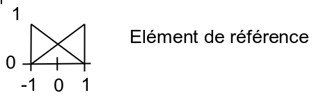
The**shape functions* of node \(k\) of \({\Gamma }_{0}:{\phi }_{k}(s)(1\le k\le \mathrm{NNO}=\text{nombre de noeuds de}{\Gamma }_{0})\) (degree one for linear elements and degree two for quadratic elements).
Recall that Legendre polynomials are a non-standardized orthogonal family. They are obtained by the recurrence relationship:
\((n+1){P}_{n+1}(t)-(\mathrm{2n}+1)t{P}_{n}(t)+n{P}_{n-1}(t)=0\)
In particular:
\(\begin{array}{}{P}_{0}(t)=1\\ {P}_{1}(t)=t\\ {P}_{2}(t)=\frac{({\mathrm{3t}}^{2}-1)}{2}\\ {P}_{3}(t)=\frac{({\mathrm{5t}}^{3}-\mathrm{3t})}{2}\end{array}\)
They are standardized in the form:
\({\gamma }_{j}(s)=\sqrt{\frac{\mathrm{2j}+1}{l}}{P}_{j}(\frac{\mathrm{2s}}{l}-1)\)
where:
\(s\) is the curvilinear abscissa of \({\Gamma }_{0}\),
\(l\) the length of the bottom of the \({\Gamma }_{0}\) crack.
Figure 2.3-b: Legend Polynomials
We limit ourselves to \({\mathrm{Deg}}_{\mathrm{max}}=7\) as the maximum degree.
Shape functions \({\varphi }_{k}(s)\) are associated with the discretization of \({\Gamma }_{0}\).
Figure 2.3-c: Crack bottom shape functions (linear elements)
Remember that we have to discretize \(G(s)\) along the bottom of the crack:
\(G(s)=\sum _{j=1}^{N}{G}_{j}{p}_{j}(s)\)
and to give ourselves a base of \({(\stackrel{ˉ}{{\theta }^{i}}(s))}_{1\le i\le N}\) test functions for the trace of field \(\theta\) on the background of crack \({\Gamma }_{0}\).
There are therefore several possible discretization options, summarized in the table below:
Polynomials of LEGENDRE |
Shape Functions |
|
\(G(s)\) |
|
|
\(\stackrel{ˉ}{\theta }(s)\) |
|
|
Table 2.3-1: Discretization choice
\(\mathrm{NNO}\) |
: |
number of nodes at the bottom of the crack \({\Gamma }_{0}\) |
\(\mathrm{NDEG}\) |
: |
maximum degree of Legender polynomials chosen by user \(\mathrm{NDEG}\le {\mathrm{Deg}}_{\mathrm{max}}=7\) |
In the CALC_G command (see [U4.82.03]) the keywords LISSAGE_THETA and LISSAGE_G allow you to choose the discretization of \(\stackrel{ˉ}{\theta }\) and \(G(s)\).
The options available are summarized in the following table:
\(\stackrel{ˉ}{\theta }(s)\) |
|||
Polynomials of Legendre |
Shape features |
||
\(G(s)\) |
Polynomials of Legendre |
LISSAGE_THETA = “LEGENDRE” LISSAGE_G = “LEGENDRE” (1st case) |
LISSAGE_THETA = “LAGRANGE” LISSAGE_G = “LEGENDRE” (2nd case) |
Shape features |
Not available |
LISSAGE_THETA = “LAGRANGE” LISSAGE_G = “LAGRANGE” “” LAGRANGE_NO_NO “(3rd case) |
|
Table 2.3-2: Discretization options
2.3.2. First case (LEGENDRE - LEGENDRE)#
\(G(s)\) is decomposed according to Legendre polynomials:
\(G(s)=\sum _{j=0}^{\mathrm{NDEG}}{G}_{j}{\gamma }_{j}(s)\)
The basis of the test functions for \(\theta (s)\) is defined using Legendre polynomials: \(\theta (s)\)
\(\tilde{\Theta }=\{{\theta }^{i}\in \Theta :\stackrel{ˉ}{{\theta }^{i}}(s)\mathrm{.}m(s)={\varphi }_{i}(s),i=\mathrm{1,}\mathrm{...},\mathrm{NDEG}\}\)
The \(\mathrm{NDEG}\) \({G}_{j}\) components are determined by solving the linear system with \(\mathrm{NDEG}\) equations:
\(\{\begin{array}{}\sum _{j=0}^{\mathrm{NDEG}}{a}_{\mathrm{ij}}{G}_{j}={b}_{i},i=\mathrm{1,}\mathrm{NDEG}\\ \text{avec}\{\begin{array}{}{a}_{\mathrm{ij}}=\underset{{\Gamma }_{0}}{\int }{\gamma }_{i}(s){\gamma }_{j}(s)\mathrm{ds}\\ {b}_{i}=G({\theta }^{i})\end{array}\end{array}\)
Since the Legendre polynomials form an orthonormal base on \({\Gamma }_{0}\), we have \({a}_{\mathrm{ij}}={\delta }_{\mathrm{ij}}\) and the linear system is therefore reduced to:
\({G}_{j}=G({\theta }^{j})\) and therefore \(G(s)=\sum _{j=0}^{\mathrm{NDEG}}G({\theta }^{j}){\gamma }_{j}(s)\).
2.3.3. Second case (LEGENDRE - LAGRANGE)#
\(G(s)\) is decomposed according to Legendre polynomials:
\(G(s)=\sum _{j=0}^{\mathrm{NDEG}}{G}_{j}{\gamma }_{j}(s)\)
The basis of the test functions for \(\theta (s)\) is defined based on the shape functions of the \(\mathrm{NNO}\) nodes of the crack bottom:
\(\tilde{\Theta }=\{{\theta }^{i}\in \Theta :\stackrel{ˉ}{{\theta }^{i}}(s)\mathrm{.}m(s)={\varphi }_{i}(s),i=\mathrm{1,}\mathrm{...},\mathrm{NNO}\}\)
where \({\varphi }_{i}(s)\) is the function of the shape of the \(i\) node at the bottom of the crack.
We then have \(\mathrm{NNO}\) equations with \(\mathrm{NDEG}\) unknowns:
\(\{\begin{array}{c}\sum _{j=0}^{\mathit{NNO}}{a}_{\mathit{ij}}{G}_{j}={b}_{i},i=1,\mathit{NNO}\\ \text{avec}\{\begin{array}{c}{a}_{\mathit{ij}}=\underset{{\mathrm{\Gamma }}_{0}}{\int }{\mathrm{\gamma }}_{j}(s){\mathrm{\phi }}_{i}(s)\mathit{ds}\\ {b}_{i}=G({\mathrm{\theta }}^{i})\hfill \end{array}\end{array}\)
In this case, we must have \(\mathrm{NDEG}\le \mathrm{NNO}\) , either \(\mathrm{NDEG}<\mathrm{min}(\mathrm{7,}\mathrm{NNO})\) where \(\mathrm{NNO}\) is the number of nodes at the bottom of the crack.
2.3.4. Third case (LAGRANGE - LAGRANGE)#
\(G(s)\) is defined by the shape functions of the \(\mathrm{NNO}\) nodes at the crack bottom:
\(G(s)=\sum _{j=0}^{\mathrm{NNO}}{G}_{j}{\varphi }_{j}(s)\)
The basis of the test functions for \(\theta (s)\) is defined based on the shape functions of the \(\mathrm{NNO}\) nodes of the crack bottom:
\(\tilde{\Theta }=\{{\theta }^{i}\in \Theta :\stackrel{ˉ}{{\theta }^{i}}(s)\mathrm{.}m(s)={\varphi }_{i}(s),i=\mathrm{1,}\mathrm{...},\mathrm{NNO}\}\)
where \({\varphi }_{i}(s)\) is the function of the shape of the \(i\) node at the bottom of the crack.
The system to be solved is as follows:
\(\{\begin{array}{c}\sum _{j=0}^{\mathit{NNO}}{a}_{\mathit{ij}}{G}_{j}=G({\mathrm{\theta }}^{i})\phantom{\rule{4em}{0ex}}(i=\mathrm{1,.}\mathrm{..},\mathit{NNO})\\ \text{avec}{a}_{\mathit{ij}}=\underset{{\mathrm{\Gamma }}_{0}}{\int }{\mathrm{\phi }}_{i}(s){\mathrm{\phi }}_{j}(s)\mathit{ds}\hfill \end{array}\)
Linear elements:
If we have linear elements:
\(\begin{array}{}{\varphi }_{1}(x)=\frac{1}{2}(1-x)\\ {\varphi }_{2}(x)=\frac{1}{2}(1+x)\end{array}\) |
|
\(\begin{array}{ccc}{a}_{i(i-j)}& \text{=}& {a}_{i,(i+j)}\text{=}0\text{, si}j\ge 2\\ {a}_{i(i-1)}& \text{=}& \underset{{\Gamma }_{0}}{\int }{\varphi }_{i}(s){\varphi }_{i-1}(s)\mathrm{ds}=\underset{{s}_{i-1}}{\overset{{s}_{i}}{\int }}{\varphi }_{i}(s){\varphi }_{i-1}(s)\mathrm{ds}\\ \text{}& \text{=}& \frac{{s}_{i}-{s}_{i-1}}{2}\underset{-1}{\overset{+1}{\int }}{\varphi }_{i}(x){\varphi }_{i-1}(x)\mathrm{dx}=\frac{{s}_{i}-{s}_{i-1}}{2}\underset{-1}{\overset{+1}{\int }}\frac{1}{4}(1-{x}^{2})\mathrm{dx}=\frac{1}{6}({s}_{i}-{s}_{i-1})\\ {a}_{\mathrm{ii}}& \text{=}& \frac{{s}_{i}-{s}_{i-1}}{2}\underset{-1}{\overset{+1}{\int }}{\varphi }_{2}^{2}(x)\mathrm{dx}+\frac{{s}_{i+1}-{s}_{i}}{2}\underset{-1}{\overset{+1}{\int }}{\varphi }_{1}^{2}(x)\mathrm{dx}\\ \text{}& \text{=}& \frac{{s}_{i}-{s}_{i-1}}{2}\underset{-1}{\overset{+1}{\int }}\frac{1}{4}{(1+x)}^{2}\mathrm{dx}+\frac{{s}_{i+1}-{s}_{i}}{2}\underset{-1}{\overset{+1}{\int }}\frac{1}{4}{(1-x)}^{2}\mathrm{dx}=\frac{1}{3}\left[({s}_{i+1}-{s}_{i})+({s}_{i}-{s}_{i-1})\right]\end{array}\)
Figure 2.3-d: Linear form functions
In the case of an open background, the matrix \({A}_{\mathit{ij}}\) is therefore written:
\(\frac{1}{6}\left(\begin{array}{ccccccc}2({s}_{2}-{s}_{1})& ({s}_{2}-{s}_{1})& 0& 0& \text{...}& 0& 0\\ ({s}_{2}-{s}_{1})& 2({s}_{3}-{s}_{1})& ({s}_{3}-{s}_{2})& 0& \text{...}& 0& 0\\ 0& ({s}_{3}-{s}_{2})& 2({s}_{4}-{s}_{2})& ({s}_{4}-{s}_{3})& \text{...}& 0& 0\\ 0& 0& ({s}_{4}-{s}_{3})& 2({s}_{5}-{s}_{3})& \text{...}& 0& 0\\ \text{...}& \text{...}& \text{...}& \text{...}& \text{...}& \text{...}& \text{...}\\ 0& 0& 0& 0& \text{...}& 2({s}_{n}-{s}_{n-2})& ({s}_{n}-{s}_{n-1})\\ 0& 0& 0& 0& \text{...}& ({s}_{n}-{s}_{n-1})& 2({s}_{n}-{s}_{n-1})\end{array}\right)\)
On the other hand, in the case of a closed background, the condition on the second member \({b}_{1}={b}_{\mathit{NNO}}\) implies that \({G}_{1}={G}_{\mathit{NNO}}\).
To get that \({G}_{1}={G}_{\mathit{NNO}}\), you need to add terms to the matrix of the linear system \({A}_{\mathrm{ij}}\) on the first and last rows.
\(\frac{1}{6}\left(\begin{array}{ccccccc}2({s}_{2}-{s}_{1})+2({s}_{n}-{s}_{n-1})& ({s}_{2}-{s}_{1})& 0& 0& \mathrm{...}& ({s}_{n}-{s}_{n-1})& 0\\ ({s}_{2}-{s}_{1})& 2({s}_{3}-{s}_{1})& ({s}_{3}-{s}_{2})& 0& \mathrm{...}& 0& 0\\ 0& ({s}_{3}-{s}_{2})& 2({s}_{4}-{s}_{2})& ({s}_{4}-{s}_{3})& \mathrm{...}& 0& 0\\ 0& 0& ({s}_{4}-{s}_{3})& 2({s}_{5}-{s}_{3})& \mathrm{...}& 0& 0\\ \mathrm{...}& \mathrm{...}& \mathrm{...}& \mathrm{...}& \mathrm{...}& \mathrm{...}& \mathrm{...}\\ 0& 0& 0& 0& \mathrm{...}& 2({s}_{n}-{s}_{n-2})& ({s}_{n}-{s}_{n-1})\\ 0& ({s}_{2}-{s}_{1})& 0& 0& \mathrm{...}& ({s}_{n}-{s}_{n-1})& 2({s}_{2}-{s}_{1})+2({s}_{n}-{s}_{n-1})\end{array}\right)\)
Quadratic elements:
If we have quadratic elements:
\(\begin{array}{}{\varphi }_{1}(x)=\frac{1}{2}x(x-1)\\ {\varphi }_{2}(x)=\frac{1}{2}x(x+1)\\ {\varphi }_{3}(x)=(1-x)(1+x)\end{array}\)
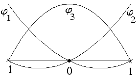
Figure 2.3-e: Quadratic Form Functions (Reference Item)
A distinction must be made between the top node and the middle node.
\(i\) = summit node:
\(\begin{array}{ccc}{a}_{i(i-j)}& \text{=}& {a}_{i,(i+j)}\text{=}0\text{, si}j\ge 3\\ {a}_{i(i-2)}& \text{=}& \underset{{\Gamma }_{0}}{\int }{\varphi }_{i}(s){\varphi }_{i-2}(s)\mathrm{ds}=\underset{{s}_{i-2}}{\overset{{s}_{i}}{\int }}{\varphi }_{i}(s){\varphi }_{i-2}(s)\mathrm{ds}\\ \text{}& \text{=}& \frac{({s}_{i}-{s}_{i-2})}{2}\underset{-1}{\overset{+1}{\int }}{\varphi }_{1}(x){\varphi }_{2}(x)\mathrm{dx}=\frac{({s}_{i}-{s}_{i-2})}{2}\underset{-1}{\overset{+1}{\int }}\frac{1}{4}{x}^{2}({x}^{2}-1)\mathrm{dx}\\ \text{}& \text{=}& -\frac{({s}_{i}-{s}_{i-2})}{30}\\ {a}_{i(i-1)}& \text{=}& \underset{{\Gamma }_{0}}{\int }{\varphi }_{i}(s){\varphi }_{i-1}(s)\mathrm{ds}=\underset{{s}_{i-2}}{\overset{{s}_{i}}{\int }}{\varphi }_{i}(s){\varphi }_{i-1}(s)\mathrm{ds}=\frac{({s}_{i}-{s}_{i-2})}{2}\underset{-1}{\overset{+1}{\int }}{\varphi }_{2}(x){\varphi }_{3}(x)\mathrm{dx}\\ \text{}& \text{=}& \frac{({s}_{i}-{s}_{i-2})}{2}\underset{-1}{\overset{+1}{\int }}\frac{1}{2}x{(x+1)}^{2}(1-x)\mathrm{dx}=\frac{({s}_{i}-{s}_{i-2})}{15}\\ {a}_{\mathrm{ii}}& \text{=}& \frac{{s}_{i}-{s}_{i-2}}{2}\underset{-1}{\overset{+1}{\int }}{\varphi }_{2}^{2}(x)\mathrm{dx}+\frac{{s}_{i+2}-{s}_{i}}{2}\underset{-1}{\overset{+1}{\int }}{\varphi }_{1}^{2}(x)\mathrm{dx}=\frac{2}{15}({s}_{i+2}-{s}_{i-2})\end{array}\)
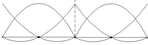
Figure 2.3-f: Summit node
\(i\) = middle node:
\(\begin{array}{ccc}{a}_{i(i-j)}& \text{=}& {a}_{i,(i+j)}\text{=}0\text{, si}j\ge 2\\ {a}_{i(i-1)}& \text{=}& \underset{-1}{\overset{+1}{\int }}\frac{({s}_{i+1}-{s}_{i-1})}{2}{\varphi }_{3}(x){\varphi }_{1}(x)\mathrm{dx}=\frac{({s}_{i+1}-{s}_{i-1})}{2}\underset{-1}{\overset{+1}{\int }}\frac{1}{2}x(x-1)(1-x)(1+x)\mathrm{dx}\\ \text{}& \text{=}& \frac{({s}_{i+1}-{s}_{i-1})}{15}\\ {a}_{\mathrm{ii}}& \text{=}& \underset{{s}_{i-1}}{\overset{{s}_{i+1}}{\int }}{\varphi }_{i}^{2}(s)\mathrm{ds}=\frac{({s}_{i+1}-{s}_{i})}{2}\underset{-1}{\overset{+1}{\int }}{(1-x)}^{2}{(1+x)}^{2}\mathrm{dx}=\frac{8}{15}({s}_{i+1}-{s}_{i-1})\end{array}\)
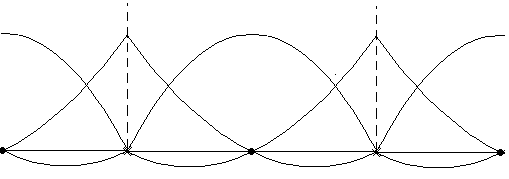
Figure 2.3-g: Middle knot
Matrix \({A}_{\mathit{ij}}\) is written as:
\(\frac{1}{30}\left(\begin{array}{ccccccc}4({s}_{3}-{s}_{1})& 2({s}_{3}-{s}_{1})& -({s}_{3}-{s}_{1})& 0& 0& \text{...}& 0\\ 2({s}_{3}-{s}_{1})& 16({s}_{3}-{s}_{1})& 2({s}_{3}-{s}_{1})& 0& 0& \text{...}& 0\\ -({s}_{3}-{s}_{1})& 2({s}_{3}-{s}_{1})& 4({s}_{5}-{s}_{1})& 2({s}_{5}-{s}_{3})& -({s}_{5}-{s}_{3})& \text{...}& 0\\ 0& 0& 2({s}_{5}-{s}_{3})& 16({s}_{5}-{s}_{3})& 2({s}_{5}-{s}_{3})& \text{...}& 0\\ 0& 0& -({s}_{5}-{s}_{3})& 2({s}_{5}-{s}_{3})& 4({s}_{7}-{s}_{3})& \text{...}& 0\\ \text{...}& \text{...}& \text{...}& \text{...}& \text{...}& \text{...}& \text{...}\\ 0& 0& 0& 0& 0& \text{...}& -({s}_{n}-{s}_{n-2})\\ 0& 0& 0& 0& 0& \text{...}& 2({s}_{n}-{s}_{n-2})\\ 0& 0& 0& 0& 0& \text{...}& 4({s}_{n}-{s}_{n-2})\end{array}\right)\)
Special case: \({s}_{i+2}-{s}_{i}=\mathrm{cste}=l=\text{longueur d’un élément}\) |
\(\frac{l}{30}\left(\begin{array}{cccccc}4& 2& -1& 0& 0& \mathrm{...}\\ 2& 16& 2& 0& 0& \mathrm{...}\\ -1& 2& 8& 2& -1& \mathrm{...}\\ 0& 0& 2& 16& 2& \mathrm{...}\\ 0& 0& -1& 2& 8& \mathrm{...}\\ \mathrm{.}& \mathrm{.}& \phantom{\rule{2em}{0ex}}& \phantom{\rule{2em}{0ex}}& \phantom{\rule{2em}{0ex}}& \phantom{\rule{2em}{0ex}}\\ \mathrm{.}& \mathrm{.}& \phantom{\rule{2em}{0ex}}& \phantom{\rule{2em}{0ex}}& \phantom{\rule{2em}{0ex}}& \phantom{\rule{2em}{0ex}}\\ \mathrm{.}& \mathrm{.}& \phantom{\rule{2em}{0ex}}& \phantom{\rule{2em}{0ex}}& \phantom{\rule{2em}{0ex}}& \phantom{\rule{2em}{0ex}}\end{array}\right)\begin{array}{c}\leftarrow \text{noeud sommet de bord}\hfill \\ \leftarrow \text{noeud milieu}\hfill \\ \leftarrow \text{noeud sommet}\hfill \\ \mathrm{.}\\ \mathrm{.}\\ \mathrm{.}\\ \mathrm{.}\\ \mathrm{.}\end{array}\)
In the case of a closed background, terms are added to the matrix of the linear system to respect condition \({G}_{1}={G}_{\mathit{NNO}}\). Matrix \({A}_{\mathrm{ij}}\) is written as:
\(\frac{1}{30}\left(\begin{array}{cccccccc}4({s}_{3}-{s}_{1})+4({s}_{n}-{s}_{n-2})& 2({s}_{3}-{s}_{1})& -({s}_{3}-{s}_{1})& 0& \mathrm{...}& -({s}_{n}-{s}_{n-1})& 2({s}_{n}-{s}_{n-2})& 0\\ 2({s}_{3}-{s}_{1})& 16({s}_{3}-{s}_{1})& 2({s}_{3}-{s}_{1})& 0& 0& \mathrm{...}& 0& 0\\ -({s}_{3}-{s}_{1})& 2({s}_{3}-{s}_{1})& 4({s}_{5}-{s}_{1})& 2({s}_{5}-{s}_{3})& -({s}_{5}-{s}_{3})& 0& \mathrm{...}& 0\\ 0& 0& 2({s}_{5}-{s}_{3})& 16({s}_{5}-{s}_{3})& 2({s}_{5}-{s}_{3})& 0& \mathrm{...}& 0\\ 0& 0& -({s}_{5}-{s}_{3})& 2({s}_{5}-{s}_{3})& 4({s}_{7}-{s}_{3})& 0& \mathrm{...}& 0\\ \mathrm{...}& \mathrm{...}& \mathrm{...}& \mathrm{...}& \mathrm{...}& \mathrm{...}& \mathrm{...}& \mathrm{...}\\ 0& 0& 0& 0& 0& 0& \mathrm{...}& -({s}_{n}-{s}_{n-2})\\ 0& 0& 0& 0& 0& 0& \mathrm{...}& 2({s}_{n}-{s}_{n-2})\\ 0& 2({s}_{3}-{s}_{1})& -({s}_{3}-{s}_{1})& 0& 0& 0& \mathrm{...}& 4({s}_{3}-{s}_{1})+4({s}_{n}-{s}_{n-2})\end{array}\right)\)
2.3.5. Third case (LAGRANGE_NO_NO - LAGRANGE)#
This method comes from the Lagrange-Lagrange method but it is simplified: the resolution of the linear system is replaced by multiplying the \(G({\theta }^{i})\) values by a weighting coefficient.
\({G}_{i}={\alpha }_{i}G({\theta }^{i})\)
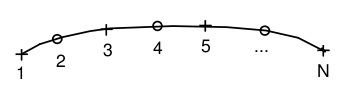
Figure 2.3-h: « Node-by-Node » Method
In addition, if \(G({\theta }^{i})=\mathrm{cste}=b,\forall i\) and we consider a constant \(G\) per element (this method has no vector meaning), we have:
vertex edge node: \(\frac{l}{30}(4+2\mathrm{-}1)G\mathrm{=}b\) or \(G\mathrm{=}\frac{6}{l}b\)
vertex node: \(\frac{l}{30}(\mathrm{-}1+2+2+8\mathrm{-}1)G\mathrm{=}b\) or \(G\mathrm{=}\frac{3}{l}b\)

middle node: \(\frac{l}{30}(2+16+2)G\mathrm{=}b\) or \(G\mathrm{=}\frac{3}{\mathrm{2l}}b\)
This gives in the case where the elements do not have constant lengths:
vertex edge node: \({\mathrm{\alpha }}_{1}=\frac{6}{({s}_{3}-{s}_{1})}\) or \({\alpha }_{N}\mathrm{=}\frac{6}{({s}_{N}\mathrm{-}{s}_{N\mathrm{-}2})}\)
vertex node: for example \({\alpha }_{3}=\frac{6}{({s}_{3}-{s}_{1})+({s}_{5}-{s}_{3})}=\frac{6}{({s}_{5}-{s}_{1})}\)
That is: \({\alpha }_{i}=\frac{6}{({s}_{i+2}-{s}_{i-2})}\)
or again: \({\alpha }_{i}^{\text{'}}\mathrm{=}\frac{3}{({s}_{i+1}\mathrm{-}{s}_{i})}\mathrm{\approx }{\alpha }_{i}\)
middle knot: \({\alpha }_{i}=\frac{3}{2({s}_{i+1}-{s}_{i})}\)
To activate this method you must specify in CALC_G:
LISSAGE_G = 'LAGRANGE_NO_NO'

LISSAGE_THETA = 'LAGRANGE'
2.3.6. Correction of values at the ends of the crack bottom#
When the bottom of the crack opens, a special additional treatment is carried out.
It has been observed for Lagrange-type smoothings (and its variants) that the numerical values of :math:`` for \(i\mathrm{=}1\) and \(i\mathrm{=}n\) are particular « false ». This is probably due to the order of the singularity that is no longer in \(-1/2\) near free surfaces. In fact, the order of the singularity at the edges depends on \(\nu\) (and on the angle between the crack bottom and the free surface and on the angle between the normal to the crack surface and the normal to the free surface). Even for a crack in a plane orthogonal to the free surface and emerging orthogonally, the singularity is not \(-1/2\) if \(\nu \mathrm{\ne }0\).
In order to improve the results at the edge points, we modify the \(G({\theta }^{i})\) for \(i\mathrm{=}1\) and \(i\mathrm{=}n\) for the smoothing of LAGRANGE - LAGRANGE and a direct modification of the \(G({s}_{i})\) for \(i\mathrm{=}1\) and \(i\mathrm{=}n\) for the LAGRANGE_NO_NO - LAGRANGE for the -, only for the option CALC_K_G. We also change \({K}_{j}({\theta }^{i})\), \(j\mathrm{=}I,\mathit{II},\mathit{III}\). This treatment is done even if symmetry conditions are applied to the edges of the background (whereas in this case, the order of the singularity is in \(-1/2\) and no treatment would be necessary).
Smoothing LAGRANGE - LAGRANGE and linear meshes
We’re making the assumption that \(G({s}_{1})\mathrm{=}G({s}_{2})\mathrm{=}G({s}_{3})\mathrm{=}{G}_{a}\) and \(G({s}_{n})\mathrm{=}G({s}_{n\mathrm{-}1})\mathrm{=}G({s}_{n\mathrm{-}2})\mathrm{=}{G}_{b}\). So by multiplying the matrix \(A\) by the vector \(G(s)\) we get:
\(G({\theta }^{1})\mathrm{=}\frac{1}{2}({s}_{2}\mathrm{-}{s}_{1}){G}_{a}\)
\(G({\theta }^{2})\mathrm{=}\frac{1}{2}({s}_{3}\mathrm{-}{s}_{1}){G}_{a}\)
…
\(G({\theta }^{n\mathrm{-}1})\mathrm{=}\frac{1}{2}({s}_{n}\mathrm{-}{s}_{n\mathrm{-}2}){G}_{b}\)
\(G({\theta }^{n})\mathrm{=}\frac{1}{2}({s}_{n}\mathrm{-}{s}_{n\mathrm{-}1}){G}_{b}\)
Let’s say \(G({\theta }^{1})\mathrm{=}G({\theta }^{2})\frac{({s}_{2}\mathrm{-}{s}_{1})}{({s}_{3}\mathrm{-}{s}_{1})}\) and \(G({\theta }^{n})\mathrm{=}G({\theta }^{n\mathrm{-}1})\frac{({s}_{n}\mathrm{-}{s}_{n\mathrm{-}1})}{({s}_{n}\mathrm{-}{s}_{n\mathrm{-}2})}\)
Smoothing LAGRANGE - LAGRANGE and quadratic meshes
We’re making the assumption that \(G({s}_{1})\mathrm{=}G({s}_{2})\mathrm{=}G({s}_{3})\mathrm{=}{G}_{a}\) and \(G({s}_{n})\mathrm{=}G({s}_{n\mathrm{-}1})\mathrm{=}G({s}_{n\mathrm{-}2})\mathrm{=}{G}_{b}\). So by multiplying the matrix \(A\) by the vector \(G(s)\) we get:
\(G({\theta }^{1})\mathrm{=}\frac{1}{6}({s}_{3}\mathrm{-}{s}_{1}){G}_{a}\)
\(G({\theta }^{2})\mathrm{=}\frac{4}{6}({s}_{3}\mathrm{-}{s}_{1}){G}_{a}\)
…
\(G({\theta }^{n\mathrm{-}1})\mathrm{=}\frac{4}{6}({s}_{n}\mathrm{-}{s}_{n\mathrm{-}2}){G}_{b}\)
\(G({\theta }^{n})\mathrm{=}\frac{4}{6}({s}_{n}\mathrm{-}{s}_{n\mathrm{-}2}){G}_{b}\)
Let’s say \(G({\theta }^{1})\mathrm{=}\frac{1}{4}G({\theta }^{2})\) and \(G({\theta }^{n})\mathrm{=}\frac{1}{4}G({\theta }^{n\mathrm{-}1})\)
Smoothing LAGRANGE_NO_NO - LAGRANGE
A linear extrapolation is made between the 2nd and 3rd bottom points (resp. between the 2 penultimate bottom points). Either:
\(G({s}_{1})\mathrm{=}G({s}_{2})+\frac{({s}_{1}\mathrm{-}{s}_{2})}{({s}_{3}\mathrm{-}{s}_{2})}(G({s}_{3})\mathrm{-}G({s}_{2}))\) and \(G({s}_{n})\mathrm{=}G({s}_{n\mathrm{-}1})\frac{({s}_{n}\mathrm{-}{s}_{n\mathrm{-}1})}{({s}_{n\mathrm{-}2}\mathrm{-}{s}_{n\mathrm{-}1})}(G({s}_{n\mathrm{-}2})\mathrm{-}G({s}_{n\mathrm{-}1}))\)
2.4. G implantation in linear thermoelasticity#
2.4.1. Types of items and loads#
It is possible to calculate the energy restoration rate in linear thermoelasticity in 2D \((G(\theta ))\) and in 3D (local value \(G(s)\)) using the CALC_G [U4.82.03] command.
The virtual propagation field of crack \(\theta\) is automatically calculated in the CALC_G command based on information provided by the user.
These calculations are valid for the following models:
D_ PLAN (meshed or non-meshed crack)
C_ PLAN (meshed or non-meshed crack)
AXIS (meshed or non-meshed crack)
3D (meshed or non-meshed crack)
and for the following thermo-mechanical loads:
\(f\), field of volume forces applied to \(\Omega\) (mechanical loads of the type PESANTEUR, ROTATION, FORCE_INTERNE),
\(g\), field of surface forces applied to part \(S\) of \(\delta \Omega\) (including on the lips of the crack: PRES_REP, FORCE_FACE),
\(T\), temperature field (transmitted via the material field: AFFE_MATERIAU/AFFE_VARC),
\({\varepsilon }^{0}\), pre-deformation field (PRE_EPSI).
These loads may depend on time and space. We do not take into account the term due to the movements imposed on \({S}_{d}\), so we should not impose Dirichlet conditions on the lips of the crack.
The characteristics of the material \((E,\nu ,\alpha )\) may depend on temperature \(T\) and space while remaining constant by elements.
In addition, a initial constraint \({\sigma }^{0}\) field can be taken into account.
2.4.2. Necessary environment#
Mesh crack:
To calculate the restoration rate (option CALC_G), it is necessary to first characterize the crack using the fond_fiss concept (in 3D: ordered list of bottom nodes, meshes of the upper lip and the lower lip; in 2D: node at the bottom of the crack and normal to the crack), with the command DEFI_FOND_FISS [U4.82.01].
When the crack is arranged along an axis of symmetry, we can content ourselves with representing only half of the model, and specify the symmetry of the load with the keyword SYME in DEFI_FOND_FISS. By default, it is assumed that there is no symmetry. If the model has symmetry, CALC_G automatically detects it using the fond_fiss concept.
Unmeshed crack (method X- FEM) :
In 2D as in 3D, the crack must be defined, for mechanical calculation and for post-processing, using the DEFI_FISS_XFEM command. The FISSURE keyword must be entered in CALC_G.
If the crack is not meshed, it is not possible to take into account the possible symmetries of the model with respect to the lips of the crack.
The calculation of \(G\) is done in post-processing, only from the displacement field solution of the calculation on the model in question. In particular, the free energy density and the stresses are calculated from the displacement field and the characteristics of the material.
2.4.3. Calculations of the different terms of the energy return rate#
The full expression for \(G(\theta )\) is given in [§1.3]. We are going to detail each term. Field \(\theta\) is zero outside of a disk with radius \({R}_{\text{sup}}(s)\) defined in chapter 3 [Figure 3.3-a]. Note that as all terms involve \(\theta\) or its gradient, the elementary terms are zero outside of this disk of radius \({R}_{\text{sup}}(s)\). In the CALC_G command, it is therefore not necessary to specify the loads that do not apply in this area.
2.4.3.1. Elementary classical term#
\(\mathrm{TCLA}={\sigma }_{\mathrm{ij}}{u}_{i,p}{\theta }_{p,j}-\psi (\varepsilon (u),T){\theta }_{k,k}\)
Elastic energy density \(\Psi (\varepsilon (u),T)\) is written in linear thermoelasticity:
in 3D and in AXIS:
\(\Psi (\varepsilon (u),T)=\frac{1}{2}\lambda {({\varepsilon }_{\mathrm{ii}})}^{2}+\mu {\varepsilon }_{\mathrm{ij}}{\varepsilon }_{\mathrm{ij}}-{\psi }_{\mathrm{th}}\)
in plane deformations:
\(\Psi (\varepsilon (u),T)=\frac{(1-\nu )E}{2(1+\nu )(1-2\nu )}({\varepsilon }_{\mathrm{xx}}^{2}+{\varepsilon }_{\mathrm{yy}}^{2})+\frac{\nu E}{(1+\nu )(1-2\nu )}{\varepsilon }_{\mathrm{xx}}{\varepsilon }_{\mathrm{yy}}+\frac{E}{(1+\nu )}{\varepsilon }_{\mathrm{xy}}^{2}-{\psi }_{\mathrm{th}}\)
in plane constraints:
\(\Psi (\varepsilon (u),T)=\frac{E}{2(1-{\nu }^{2})}({\varepsilon }_{\mathrm{xx}}^{2}+{\varepsilon }_{\mathrm{yy}}^{2})+\frac{\nu E}{(1-{\nu }^{2})}{\varepsilon }_{\mathrm{xx}}{\varepsilon }_{\mathrm{yy}}+\frac{E}{(1+\nu )}{\varepsilon }_{\mathrm{xy}}^{2}-{\psi }_{\mathrm{th}}\)
with \({\Psi }_{\mathrm{th}}=\mathrm{3K}\alpha (T-{T}_{\mathrm{réf}}){\varepsilon }_{\mathrm{ii}}-\frac{9}{2}K{\alpha }^{2}{(T-{T}_{\mathrm{réf}})}^{2}\)
where:
\(\mathrm{3K}=\frac{E}{1-2\nu };\lambda =\frac{\nu E}{(1+\nu )(1-2\nu )};2\mu =\frac{E}{1+\nu }\)
\(E\): Young’s modulus
\(\nu\): Poisson’s ratio
\(\lambda ,\mu\): Lamé coefficients
\(\alpha\): thermal expansion
The elastic energy density \(\psi (\varepsilon (u),T)\) can be written in general terms in the form:
\(\begin{array}{cc}\Psi (\varepsilon (u),T)=\frac{1}{2}K{({\varepsilon }_{\mathrm{kk}}-3\alpha (T-{T}_{\mathrm{réf}}))}^{2}+\frac{2\mu }{3}{\varepsilon }_{\mathrm{eq}}^{2}& \\ \text{avec}{\varepsilon }_{\mathrm{eq}}^{2}=\frac{3}{2}{\varepsilon }_{\mathrm{ij}}^{D}{\varepsilon }_{\mathrm{ij}}^{D}\text{et}{\varepsilon }_{\mathrm{ij}}^{D}={\varepsilon }_{\mathrm{ij}}-\frac{1}{3}{\varepsilon }_{\mathrm{kk}}{\delta }_{\mathrm{ij}}& \end{array}\)
\(\text{soit}{\varepsilon }_{\mathrm{eq}}^{2}=\frac{1}{2}(3{\varepsilon }_{\mathrm{ij}}{\varepsilon }_{\mathrm{ij}}-{\varepsilon }_{\mathrm{kk}}^{2})\)
\(\begin{array}{ccc}\text{et}\Psi (\varepsilon (u),T)& \text{=}& \frac{1}{2}K{\varepsilon }_{\mathrm{kk}}^{2}-\mathrm{3K}\alpha (T-{T}_{\mathrm{réf}}){\varepsilon }_{\mathrm{kk}}+\frac{9}{2}K{\alpha }^{2}{(T-{T}_{\mathrm{réf}})}^{2}+\mu {\varepsilon }_{\mathrm{ij}}{\varepsilon }_{\mathrm{ij}}-\frac{\mu }{3}{\varepsilon }_{\mathrm{kk}}^{2}\\ & \text{=}& \frac{\lambda }{2}{\varepsilon }_{\mathrm{kk}}^{2}+\mu {\varepsilon }_{\mathrm{ij}}{\varepsilon }_{\mathrm{ij}}-\mathrm{3K}\alpha (T-{T}_{\mathrm{réf}}){\varepsilon }_{\mathrm{kk}}+\frac{9}{2}K{\alpha }^{2}{(T-{T}_{\mathrm{réf}})}^{2}\end{array}\)
2.4.3.2. Volume force term#
\(\mathrm{TFOR}={f}_{i}{u}_{i}{\theta }_{k,k}+{f}_{i,k}{\theta }_{k}{u}_{i}\)
2.4.3.3. Surface force term#
\(\mathrm{TSUR}={g}_{i,k}{\theta }_{k}{u}_{i}+{g}_{i}{u}_{i}({\theta }_{k,k}-\frac{\partial \theta }{\partial {n}_{k}}{n}_{k})\)
Note:
In this surface term we have normal derivations at the surface that do not make sense for the skin elements used. We therefore use differential geometry and contrariant derivatives to better understand this integrand on the calculation surface.
2.4.3.4. Thermal term#
\(\mathrm{THER}=-\frac{\partial \psi }{\partial T}{T}_{,k}{\theta }_{k}\)
with: \(\frac{\partial \Psi }{\partial T}(\varepsilon (u),T)=\left[\frac{1}{2}\frac{\mathrm{dK}(T)}{\mathrm{dT}}({\varepsilon }_{\mathrm{kk}}-3\alpha (T-{T}_{\mathrm{réf}}))-\mathrm{3K}(\alpha +\frac{d\alpha (T)}{\mathrm{dT}}(T-{T}_{\mathrm{réf}}))\right]({\varepsilon }_{\mathrm{kk}}-3\alpha (T-{T}_{\mathrm{réf}}))\)
2.4.3.5. Term of pre-deformations and initial stresses#
\(\mathrm{TINI}=\left[{\sigma }_{\mathrm{ij}}{\varepsilon }_{\mathrm{ij},k}^{0}-{\Lambda }_{\mathrm{ijpq}}^{\text{-1}}{\sigma }_{\mathrm{pq}}{\sigma }_{\mathrm{ij},k}^{0}\right]{\theta }_{k}\)
We can notice that if \(\sigma =0\) then \(\mathrm{TINI}=0\)
Note 1:
Like the rest of this documentation, the presence of initial stresses is only valid in the case of elasticity, and here it is isotropic linear. To be activated, you must therefore be in an incremental behavior relationship (COMPORTEMENT) with a relationship ELAS. It is not possible to provide an initial constraints field in any other case.
Note 2:
Given the difficulty of validation, it is currently not possible to combine pre-deformations (loading under the keyword PRE - EPSI) and initial constraints (keyword SIGM_INIT of CALC_G) . G calculations in the presence of an initial state can be performed with a meshed crack or a non-meshed crack.
Note 3:
In all cases, this initial stress field must be **self-balanced, in the absence of cracks, with the only limit conditions. The user can (should…) verify that his initial stress field is legitimate by applying it in the keyword* ETAT_INITde the operator STAT_NON_LINE, with incremental elastic behavior (COMPORTEMENT, RELATION = “ELAS”), with the only limit conditions; the mechanical result must be the same stress field without additional deformations.
Note 4:
The initial stress field must have been used beforehand in the thermo-mechanical calculation. The approach for calculating the energy return rate in the presence of initial constraints is presented . Reference will also be made to the dedicated test case.
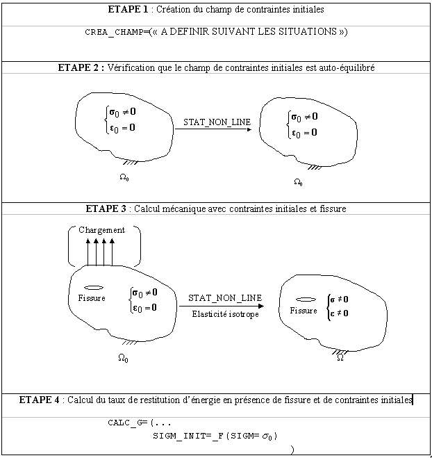
Figure 2.1: Calculation approach in the presence of initial constraints.
2.4.4. Normalization of the energy return rate#
2.4.4.1. Axisymmetry#
\(G(\theta )\) as implemented here, calculate the energy return in the kinematics defined by \(\theta\). It may need to be normalized (by hand! this is not done automatically in the code) in order to be able to compare to a value intrinsic to the material, especially axisymmetrically. Consider the case of an inclined crack, where the crack bottom is at a distance \(R\) from the axis of symmetry:
Figure 2.4.4.1-a: Axisymmetric crack bottom
Axis \(\mathrm{OY}\) is the axis of symmetry in “AXIS” modeling and the calculated energy recovery rate is:
\(G(\theta )=-\frac{\mathrm{dW}}{\mathrm{dl}}\)
where \(W\) is the potential energy per unit of radian.
However, the intrinsic value of the energy return rate is:
\(G=-\frac{{\mathrm{dW}}_{\mathrm{totale}}}{\mathrm{dA}}\)
where:
\({W}_{\mathrm{totale}}\) is the total potential energy,
\(\mathrm{dA}\) is the change in crack area.
with: \(\begin{array}{}{W}_{\mathrm{totale}}=2\pi W\\ \mathrm{dA}=2\pi R\mathrm{dl}\end{array}\)
from where: \(\frac{{\mathrm{dW}}_{\mathrm{totale}}}{\mathrm{dA}}=2\pi \frac{\mathrm{dW}}{\mathrm{dl}}\frac{\mathrm{dl}}{\mathrm{dA}}=\frac{1}{R}\frac{\mathrm{dW}}{\mathrm{dl}}\)
and therefore \(G=\frac{1}{R}G(\theta )\) in axisymmetry.
2.4.4.2. Other cases#
In dimension 2 (C_ PLAN and D_ PLAN), the crack bottom is reduced to one point and the value of \(G(\theta )\) is independent of the choice of field \(\theta\) (with \(\theta \in \Theta\) and \(\theta\) unit in the vicinity of the crack bottom).
\(G=G(\theta ),\forall \theta \in \Theta\)