2. Theoretical formulation#

2.1. State variables, state law#

The state variables are: total deformation \(\mathrm{\epsilon }\left(\mathrm{u}\right)\), plastic deformation \({\mathrm{\epsilon }}^{p}\).

Free energy density is written as:

(2.1)#\[ w\ left (\ mathrm {\ epsilon}\ left (\ mathrm {u}\ right), {\ mathrm {\ epsilon}} ^ {p}\ right) =\ frac {1} {2}\ left (\ mathrm {\ epsilon}\ left (\ mathrm {u}\ right) - {\ mathrm {\ epsilon}\ right) - {\ mathrm {\ epsilon}\ right) - {\ mathrm {\ epsilon}} ^ {p}\ right)\ mathrm {:}\ mathrm {A}\ mathrm {A}\ mathrm {:}\ left (\ mathrm {\ epsilon}\ left (\ mathrm {u}\ right) - {\ mathrm {\ epsilon}}} ^ {p}\ right)\]

where \(\mathrm{A}\) refers to the linear elasticity tensor; it is assumed to be isotropic (2 independent elastic coefficients in 3D). Work hardening is not considered.

The elastoplastic three-dimensional law of behavior is then written (state law):

(2.2)#\[ \ mathrm {\ sigma} =\ mathrm {A}\ mathrm {A}\ mathrm {:}\ left (\ mathrm {u}\ right) - {\ mathrm {\ epsilon}}} ^ {p}\ right) - {\ mathrm {\ epsilon}}} ^ {p}\ right)\]

2.2. Criterion (load area) smoothed#

The criterion delimiting the elastic domain (load surface) is formulated with the 3 tensor invariants:

(2.3)#\[ \ text {f}\ left (\ mathrm {\ sigma}\ right) =\ frac {1} {3} {I} _ {1}\ mathrm {.} \ mathrm {sin} {\ varphi} _ {\ mathit {pp}} _ {\ mathit {pp}}} +\ sqrt {{J} _ {\ varphi} _ {L}\ right) + {a}\ right) + {a} _ {\ mathit {pp}}}} +\ sqrt {{J} _ {tt}}} ^ {2} {\ varphi}\ right) + {a} _ {\ mathit {pp}}} {\ mathit {pp}}}} +\ sqrt {{J} _ {pp}}} +\ sqrt {{J} _ {pp}}} +\ sqrt {{J} _ {pp}}} +\ sqrt {{J} _ {pp}}}} +\ sqrt {{J} _ {it {pp}}} -c\ mathrm {.} \ mathrm {cos} {\ varphi} _ {\ mathit {pp}}\ phantom {\ rule {2em} {0ex}}\ phantom {\ rule {2em} {2em} {0ex}} 0\]

with \({I}_{1}=\text{tr}\left(\mathrm{\sigma }\right)=3p\) the triple of the mean pressure, \({J}_{2}=\frac{1}{2}\left({\mathrm{\sigma }}^{D}\mathrm{:}{\mathrm{\sigma }}^{D}\right)=\frac{1}{3}{\left({\Vert \mathrm{\sigma }\Vert }_{\mathit{VM}}\right)}^{2}\); \({J}_{3}=\text{det}\left({\mathrm{\sigma }}^{D}\right)\), having noted \({\mathrm{\sigma }}^{D}=\mathrm{\sigma }-p\mathrm{Id}\) the stress tensor deviator, and the modified Lode angle defined by: \({\theta }_{L}=\frac{1}{3}\mathrm{arcsin}\left(\text{-}\frac{3\sqrt{3}{J}_{3}}{2\sqrt{{J}_{2}^{3}}}\right)\phantom{\rule{2em}{0ex}}\in \phantom{\rule{2em}{0ex}}\left[\text{-}\frac{\pi }{6},\frac{\pi }{6}\right]\), and the three parameters: cohesion \(c\), the friction angle \({\varphi }_{\mathit{pp}}\), and the « traction truncation » \({a}_{\mathit{tt}}\), which is used for the approximation hyperbolic used for smoothing at the top of the Mohr-Coulomb pyramid. cf. [2].

Note 1 :

According to [2 ], if \({a}_{\mathit{tt}}=0\) , criterion (3) finds the top of the pyramid of Mohr-Coulomb, so it is no longer smoothed. if Si*:math:{a}_{mathit{tt}}=frac{1}{2}cmathrm{.}mathit{cotan}{varphi }_{mathit{pp}}`*, * ** *then at the top of the smoothed criterion, we check:* :math:`{I}_{1}=0 .

We know that the main constraints can be written according to:

\[\]

: label: eq-4

{begin {array} {c} {sigma} {sigma} _ {I} _ {1} {1} +frac {2sqrt {3}}} {3}} {3}mathrm {.} sqrt {{J} _ {2}}}mathrm {.} mathrm {sin}left ({theta} _ {L} _ {L} +frac {2pi} {3}right)\ {sigma} _ {mathit {II}}} =frac {1}}}} =frac {1}} _ {1} +frac {2sqrt {3}} {3}}mathrm {.} sqrt {{J} _ {2}}}mathrm {.} mathrm {sin}left ({theta} _ {L}right)\ {L}right)\ {sigma} _ {mathit {III}}} =frac {1} {3} {3} {3} {3} {3} {3} {3} {3} {I} _ {1} {1} {I} _ {1}} +frac {1} _ {1} +frac {1} _ {1} +frac {1} _ {1} +frac {1} _ {1} +frac {1} _ {1} +frac { sqrt {{J} _ {2}}}mathrm {.} mathrm {sin}left ({theta} _ {L} -frac {2pi} {3}right)end {array}

The \(K\left({\theta }_{L}\right)\) function in (3) is defined by:

\[\]

: label: eq-5

Kleft ({theta} _ {L}right) ={begin {array} {cc} {left (mathrm {cos} {theta} _ {L} -frac {sqrt {3}}right) ={sqrt {3}} {sqrt {3}} {3}}mathrm {3}} {3}mathrm {3}} {3}mathrm {3}} {3}mathrm {3}} {3}mathrm {3}} {3}mathrm {3}} {3}mathrm {3}} {3}mathrm {.} mathrm {sin} {theta} _ {L}right)}} ^ {2}}} ^ {2} &mathit {si}phantom {rule {2em} {0ex}}left| {theta}} _ {L}\ right} _ {L}\ right|< {L}right|< {L}right|< {L}right|< {theta} | right|< {theta} | right|< {theta} | right|< {theta} | right|< {theta} | right|< {theta} | right|< {theta} | right|< {theta} | right|< {theta} | right|< {theta}} | right|<left ({theta} _ {L}right)mathrm {.} mathrm {sin} 3 {theta} _ {L} _ {L} +Cleft ({theta} _ {L}right)mathrm {.} {mathrm {sin}} ^ {2} 3 {theta} _ {L}right)} ^ {2} &mathit {si}phantom {rule {2em} {0ex}}left| {theta}}}left| {theta}}}left| {theta} _ {theta} _ {T}end {array}}}left| {theta}}}left| {theta} _ {theta} _ {array}

with an additional \({\theta }_{T}\in \phantom{\rule{2em}{0ex}}\left[0,\frac{\pi }{6}\right]\) parameter called transition angle and \(A\left({\theta }_{L}\right),B\left({\theta }_{L}\right),C\left({\theta }_{L}\right),\) functions defined by:

(2.4)#\[\begin{split} \ {\ begin {array} {c} A\ left ({\ theta} _ {L}\ right) =\ text {-}\ frac {\ sqrt {3}} {3}\ mathrm {sin} {\ sin} {\ sin} {\ varphi} _ {\ varphi}} _ {\ mathit {pp}}\ mathrm {.} \ mathit {sgn} {\ theta} _ {L\ mathrm {.}} \ mathrm {sin} {\ theta} _ {T} -B\ left ({\ theta} _ {L}\ right)\ mathrm {.} \ mathit {sgn} {\ theta} _ {L\ mathrm {.}} \ mathrm {sin} {\ theta} _ {T} -C\ left ({\ theta} _ {L}\ right)\ mathrm {.} {\ mathrm {sin}} ^ {2} 3 {\ theta} _ {T} _ {T} +\ mathrm {cos} {\ theta} _ {T}\\ left ({\ theta} _ {L}\ right) =\ frac {\ theta}\ right) =\ frac {\ mathit {sgn}} +\ mathrm {\ theta} _ {L}\ left ({\ theta} _ {L}\ right) =\ frac {\ mathit {sgn}} {\ theta} _ {L}} \ mathrm {sin} 6 {\ theta} _ {T}\ left (\ mathrm {cos} {\ theta} _ {T} -\ frac {\ sqrt {3}}} {3\ mathrm {3}} {3\ mathrm {sin}} {\ mathrm {sin} {\ sin} {\ varphi}} _ {\ mathit {pp}}\ mathrm {.} \ mathit {sgn} {\ theta} _ {L\ mathrm {.}} \ mathrm {sin} {\ theta} _ {T}}\ right) -6\ mathrm {cos} 6 {\ theta} _ {T}\ left (\ mathit {sgn} {\ sgn} {\ theta}} _ {\ theta} _ {L\ mathrm {.}} \ mathrm {sin} {\ theta} _ {T} _ {T} +\ frac {\ sqrt {3}} {3\ mathrm {sin} {\ varphi}} _ {\ mathit {pp}}\ mathrm {.} \ mathrm {cos} {\ theta} _ {T}}\ right)} {18 {\ mathrm {cos}} ^ {3} 3 {\ theta} _ {T}}\\ C\ left ({\ theta} _ {theta} _ {L}\ right) =\ frac {-\ mathrm {cos}} 3 {\ theta} _ {T}}\ left (\ mathrm {cos} {\ theta} _ {T} -\ frac {\ sqrt {3}} {3\ mathrm {sin} {\ varphi} _ {\ mathit {pp}} -\ frac {\ sqrt {3}}}\ mathrm {.} \ mathit {sgn} {\ theta} _ {L\ mathrm {.}} \ mathrm {sin} {\ theta} _ {T}}\ right) -3\ mathit {sgn} {\ theta} _ {L}\ mathrm {sin} 3 {\ theta} _ {T} _ {T}\ left (\ mathit {sgn}} {\ theta} _ {L\ mathrm {.}} \ mathrm {sin} {\ theta} _ {T} _ {T} +\ frac {\ sqrt {3}} {3\ mathrm {sin} {\ varphi}} _ {\ mathit {pp}}\ mathrm {.} \ mathrm {cos} {\ theta} _ {T}}\ right)} {18 {\ mathrm {cos}} ^ {3} 3 {\ theta} _ {T}}}\ end {array}\end{split}\]

Note 2 :

According to [2 ], we should not take a value of \({\theta }_{T}\) too close to \(\frac{\pi }{6}\) , at the risk of poor conditioning; and a typical value of \({\theta }_{T}\) can be taken equal to \(\frac{5\pi }{36}\). With this value of . With this value of \({\theta }_{T}\) and with \({a}_{\mathit{tt}}=\frac{1}{20}c\mathrm{.}\mathit{cotan}{\varphi }_{\mathit{pp}}\) , the proposed hyperbolic smoothing leads to an error of at most 0.13% in The plan deviatory from the original Mohr-Coulomb pyramid.

The and are a graphical representation of the original Mohr-Coulomb load surface in the principal stress space. The shows the effect of smoothing [2] on the edges of the Mohr-Coulomb charge surface.

_images/100002000000018A0000011629C869B9FA99F23B.png

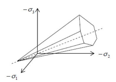
Figure 2.2-1: Representation of the Mohr-Coulomb load surface in the three-dimensional space of the main stresses.

_images/10000200000001C7000001BCB4B85E743A07E357.png

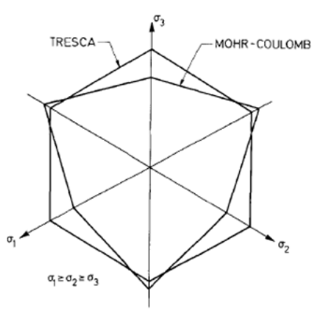
Figure 2.2-2: Representation of the Mohr-Coulomb load surface in plane \(\mathrm{\pi }\) of the stress deviators (any vector represented in this plane corresponds to a deviatoric stress).

_images/1000000000000108000000F4F8C4825CC122FB21.png

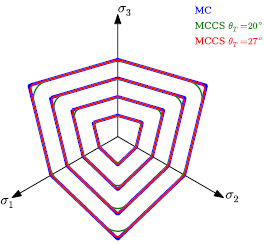
Figure 2.2-3: Representation of the Mohr-Coulomb load surface smoothed in plane \(\pi\) of the stress deviators, for the friction angle \({\varphi }_{\mathit{pp}}=25°\) and two values of \({\theta }_{T}\) (taken from [3]).

An enrichment of the criterion () is provided by adding a term for hardening to cohesion, in the following form:

(2.5)#\[ -c\ mathrm {.} \ mathrm {cos} {\ varphi} _ {\ mathit {pp}\ mathrm {.}} \ left (1+ {r} _ {\ mathit {eg}}}\ cdot {\ vert {\ epsilon} ^ {p}\ green} _ {\ mathit {VM}}}\ right)\]

where the parameter \({r}_{\mathit{eg}}\) (expressed without units) makes it possible to introduce linear cohesion work hardening.

2.3. Plastic flow potential#

The plastic flow of this law is not standard (non-associated law), and therefore not oriented according to the normal to the load surface. The authors [2] propose an expression of plastic flow using another potential with the same analytical form as that of the criterion (), by involving the dilatance angle \(\psi\):

(2.6)#\[ \ text {g}\ left (\ mathrm {\ sigma}\ right) =\ frac {1} {3} {I} _ {1}\ mathrm {.} \ mathrm {sin}\ psi +\ sqrt {{J} _ {2}\ mathrm {.} {K} _ {g}\ left ({\ theta}} _ {L}\ right) + {a} _ {\ mathit {tt}} ^ {2} {\ mathrm {tan}}} ^ {2} {2} {\ varphi}} _ {\ varphi} _ {\ mathit {pp}}\ mathrm {.}} {\ mathrm {cos}} ^ {2}\ psi} -c\ mathrm {.} \ mathrm {cos}\ psi\]

When \(\psi ={\varphi }_{\mathit{pp}}\), the law of plastic flow becomes associated.

Function \({K}_{g}\left({\theta }_{L}\right)\) in (7) is defined by:

(2.7)#\[\begin{split} {K} _ {g}\ left ({\ theta} _ {L}\ right) =\ {\ begin {array} {cc} {\ left (\ mathrm {cos} {\ theta} {\ theta} _ {L} -\ frac {\ theta} _ {L}} -\ frac {\ sqrt {3}} {L} -\ frac {\ sqrt {3}}} {3}\ mathrm {sin}\ left (\ mathrm {cos} {\ theta} {\ theta} _ {L} -\ frac {\ sqrt {3}}} {3}\ mathrm {sin}\ psi\ mathrm {.} \ mathrm {sin} {\ theta} _ {L}\ right)}} ^ {2}} &\ mathit {si}\ phantom {\ rule {2em} {0ex}}\ left| {\ theta}} _ {theta} _ {L}\\ right|< {L}\\ right|< {L}\ right|< {\ theta} | right|< {\ theta} | right|< {\ theta} _ {\ theta} _ {T}\\ left ({A} _ {\ text {g}}}\ left ({\ theta}}\ left ({\ theta}}} _ {L}\ right) + {B} _ {\ text {g}}\ left ({\ theta} _ {L}\ right)\ mathrm {.} \ mathrm {sin} 3 {\ theta} _ {L} _ {L} + {L}} + {L}\ right)\ mathrm {.}\ left ({\ theta} _ {L}\ right)\ mathrm {.} {\ mathrm {sin}} ^ {2} 3 {\ theta} _ {L}\ right)} ^ {2} &\ mathit {si}\ phantom {\ rule {2em} {0ex}}\ left| {\ theta}}}\ left| {\ theta}}}\ left| {\ theta} _ {\ theta} _ {T}\ end {array}}}\ left| {\ theta}}}\ left| {\ theta} _ {\ theta} _ {array}\end{split}\]

functions \({A}_{\text{g}}\left({\theta }_{L}\right),{B}_{\text{g}}\left({\theta }_{L}\right),{C}_{\text{g}}\left({\theta }_{L}\right),\) being defined by:

(2.8)#\[\begin{split} \ {\ begin {array} {c} {A} _ {\ text {g}}}\ left ({\ theta} _ {L}\ right) =\ text {-}\ frac {\ sqrt {3}} {3}} {3} {3}\ mathrm {g}} {3}\ mathrm {sin}\ psi\ mathrm {.} \ mathit {sgn} {\ theta} _ {L\ mathrm {.}} \ mathrm {sin} {\ theta} _ {T} - {T} - {B} _ {\ text {g}}\ left ({\ theta} _ {L}\ right)\ mathrm {.} \ mathit {sgn} {\ theta} _ {L\ mathrm {.}} \ mathrm {sin} {\ theta} _ {T} _ {T} - {C} _ {\ text {g}}\ left ({\ theta} _ {L}\ right)\ mathrm {.} {\ mathrm {sin}} ^ {2} 3 {\ theta} _ {T} _ {T} +\ mathrm {cos} {\ theta} _ {\ text {g}} _ {\ text {g}}}\ left ({\ theta}}}\ left ({\ theta}}}\ left ({\ theta}}\ left ({\ theta}}\ left ({\ theta}})\ left ({\ theta}}\ left ({\ theta}}\ left ({\ theta}})\ left ({\ theta}}\ left ({\ theta}}\ left ({\ theta}})\ left ({\ theta}}\ left ({\ theta}}\ left ({\ theta}})\ left} \ mathrm {sin} 6 {\ theta} _ {T}\ left (\ mathrm {cos} {\ theta} _ {T} -\ frac {\ sqrt {3}}} {3\ mathrm {3}} {3\ mathrm {sin}\ left (\ mathrm {sin}\ left) \ mathit {sgn} {\ theta} _ {L\ mathrm {.}} \ mathrm {sin} {\ theta} _ {T}}\ right) -6\ mathrm {cos} 6 {\ theta} _ {T}\ left (\ mathit {sgn} {\ sgn} {\ theta}} _ {\ theta} _ {L\ mathrm {.}} \ mathrm {sin} {\ theta} _ {T} _ {T} +\ frac {\ sqrt {3}} {3\ mathrm {sin}\ psi\ mathrm {.} \ mathrm {cos} {\ theta} _ {T}}\ right)} {18 {\ mathrm {cos}} ^ {3} 3 {\ theta} _ {T}}\\ {C} _ {\ C} _ {\ text {g}} _ {g}}\ right)}\ left ({\ theta}}}\ right) =\ frac {-\ mathrm {cos}}}\\ {C} _ {C} _ _ {C} _ _ {C} _ _ {C} _ _ {C} _ {C} _ _ {C} _ {T}\ left (\ mathrm {cos} {\ theta} {\ theta} _ {T} -\ frac {\ sqrt {3}}} {3\ mathrm {sin}\ psi\ mathrm {.} \ mathit {sgn} {\ theta} _ {L\ mathrm {.}} \ mathrm {sin} {\ theta} _ {T}}\ right) -3\ mathit {sgn} {\ theta} _ {L}\ mathrm {sin} 3 {\ theta} _ {T} _ {T}\ left (\ mathit {sgn}} {\ theta} _ {L\ mathrm {.}} \ mathrm {sin} {\ theta} _ {T} _ {T} +\ frac {\ sqrt {3}} {3\ mathrm {sin}\ psi\ mathrm {.} \ mathrm {cos} {\ theta} _ {T}}\ right)} {18 {\ mathrm {cos}} ^ {3} 3 {\ theta} _ {T}}}\ end {array}\end{split}\]

When the stress state is on load surface \(\text{f}\left(\mathrm{\sigma }\right)=0\), the plastic deformation rate is normal to potential \(\text{g}\left(\mathrm{\sigma }\right)\) and is written with the plastic multiplier \(d\lambda\):

(2.9)#\[ d {\ mathrm {\ epsilon}}} ^ {p} =d\ lambda\ mathrm {.} \ frac {\ partial\ text {g}} {\ partial\ mathrm {\ sigma}} =d\ lambda\ mathrm {.} {\ mathrm {n}} _ {\ text {g}}\]

where the normal tensor of order two outside the surface is:

(2.10)#\[ {\ mathrm {n}} _ {\ text {g}} =\ frac {\ partial\ text {g}\ left (\ sigma\ right)} {\ partial {I} _ {1}\ left (\ sigma\ right)}\ left (\ sigma\ right)}\ cdot\ mathrm {right)}\ cdot\ mathrm {Id}} +\ left (\ sigma\ right)}\ cdot\ mathrm {Id} +\ left (\ sigma\ right)}\ cdot\ mathrm {Id} +\ left (\ sigma\ right)}\ cdot\ mathrm {Id} +\ left (\ sigma\ right)} {\ partial {right)} {\ partial {right)} J} _ {2}\ left (\ sigma\ right)}} +\ frac {\ partial\ text {g}\ left (\ sigma\ right)} {\ partial {\ theta} _ {L}}\ cdot\ frac {\ dot\ frac {\ frac {\ frac {\ frac {\ partial {\ theta}} _ {L}}} {\ partial\ theta}}} {\ partial\ theta}}} {\ partial {\ theta}}} {\ partial\ theta}} {\ left (\ sigma\ right)}\ right) {\ sigma\ right)}\ right) {\ sigma\ frac {\ frac {\ partial {\ theta}} _ {L}}}\ right) {\ sigma\ right)}\ right) {\ sigma} ^ {D} +\ frac {\ partial\ text {g}\ left (\ sigma\ right)} {\ partial {\ theta} _ {L}}\ cdot\ frac {\ partial {\ theta} _ {L} _ {L}}} {L}}} {\ partial {J}}}} {\ partial {J} _ {L}}} {\ partial {\ theta} _ {L} _ {L}}} {L}}} {\ partial {\ theta} _ {L}}} {\ partial {\ theta} _ {L}}} {L}}} {\ partial {\ theta} _ {L}}} {\ partial {\ theta} _ {L}}} {L}}} {\ partial {\ theta} _ {L}}} {sigma\ right)} {\ partial\ sigma}\]

The only true thermodynamic internal variable is the equivalent plastic deformation \({\Vert {\epsilon }^{p}\Vert }_{\mathit{VM}}\).

We naturally have \(\frac{\partial \text{g}\left(\sigma \right)}{\partial {I}_{1}\left(\sigma \right)}=\frac{1}{3}\cdot \mathrm{sin}\psi\) and we remind you that: \(\frac{\partial {J}_{2}\left(\sigma \right)}{\partial \sigma }={\sigma }^{D}\).

Note 3 :

L e flow potential chosen, in the same shape as the criterion, therefore the flow tensor of flow \({\mathrm{n}}_{\text{g}}\) , is not affected by the possible introduction of linear cohesion work hardening, cf. * () () *. In fact, the evolution of cohesion does not modify the direction normal to the faces of the pyramid \(\text{g}\left(\mathrm{\sigma }\right)=0\) .

2.4. Energy dissipation by plastic flow#

The mechanical power density dissipated by the plasticity mechanism is:

(2.11)#\[ D=\ mathrm {\ sigma}\ mathrm {:} {\ dot {\ mathrm {\ epsilon}}}} ^ {p}\]

Mechanical energy is dissipated by accumulation during the loading path.

2.5. Behavioral relationship parameters#

The parameters of the behavioral relationship are:

YoungModulus

Young’s Modulus (positive)

\(E\)

PoissonRatio

Poisson Ratio

\(\nu\)

Cohesion

Cohesion (positive or zero)

\(c\)

FrictionAngle

Friction angle (supplied in°)

\({\varphi }_{\mathit{pp}}\)

dilatancyAngle

Expansion angle (supplied in°)

\(\psi\)

TransitionAngle

Transition Lode Angle (supplied in°, less than 30°)

\({\theta }_{T}\)

TensionCutoff

Traction truncation (positive or zero)

\({a}_{\mathit{tt}}\)

HardeningCoef

Cohesion hardening (positive or zero)

\({r}_{\mathit{eg}}\)