3. Local integration of the Mohr-Coulomb law#
The plastic deformation rate is given using the Koiter formula:
Where \(m\) characterizes the number of active mechanisms, equal to one, two, or six depending on the following situations:
the final stress is located inside the load surface, the point is regular and \(m=1\);
the final constraint is located on an edge of the cone, the point is singular and \(m=2\);
the final stress is not located inside the load surface or on an edge. It is then projected to the top of the cone, the point is singular and \(m=6\);
The final stress \({\sigma }^{\text{+}}\) is calculated on the basis of an elastic prediction noted \({\sigma }^{e}\) and a correction \({\sigma }^{c}=C\mathrm{.}d{\epsilon }^{p}\) so that:
Plastic multipliers \(d{\lambda }_{j}\) are calculated by injecting equation () into equation (), which gives:
In what follows, the expressions corresponding to the various situations mentioned above are detailed. The resolution procedure is shown in the synopsis of the figure.
3.1. Cases where only one mechanism is active#
It is detected that the prediction activates a criterion when:
We have the following expression for normal:
And so:
That we put into equation (), which becomes:
From where we deduce the plastic multiplier:
Where \({\langle \rangle }_{\text{+}}\) refers to the positive part of a quantity. In the end, we get:
If we break down the plastic deformation rate into a deviatory part \(d{\varepsilon }_{v}^{p}\mathrm{=}\mathit{trace}(d{\varepsilon }^{p})\) and a spherical part \(d{e}^{p}=d{\epsilon }^{p}-\frac{d{\epsilon }_{v}^{p}}{3}1\), we have:
Consider the following expression for the equivalent deformation increment:
: label: eq-21
d {e} ^ {p} =dmathrm {lambda}sqrt {{t} ^ {2} +3}
3.2. Cases where two mechanisms are active#
3.2.1. Formulation of the solution#
We check that \({\sigma }^{\text{+}}\) obtained from the previous step () always checks:
If this is not the case, then two mechanisms should be activated in the following way:
The definition of mechanisms LEFT and RIGHT is purely conventional, and obeys the geometric logic represented in figure.
Figure 3.2.1-1: Definition of mechanisms LEFT and RIGHT
We have the following expressions for normal ones:
So:
These expressions are introduced into equation (). For mechanism LEFT, we get the following system to solve:
For mechanism RIGHT, we get:
: label: eq-27
{begin {array} {c} 4D {lambda} ^ {12}left [G+left (K+frac {G} {3}right) tsright] +2d {lambda} ^ {12} ^ {12}left}left [Glambda} ^ {12}}left [Glambda} ^ {12}left}left [G] {3}right) tsright] = {F} _ {13}left ({sigma}left ({sigma} ^ {e}right)\ 2d {lambda} ^ {13}left [Gleft (1+t+sright) +left (mathrm {2}}right)left [G+left (K+frac {G} {G} {3}right) tsright] = {F} _ {12}left ({sigma} ^ {e}right)end {array}
For algorithmic implementation, it’s nicer to rewrite () and () as follows:
With the following plastic multipliers:
For load surfaces:
: label: eq-30
{F} _ {1}mathrm {=} {F} _ {13}
The expression of \(A\):
: label: eq-31
A=4left [G+left (K+frac {G} {3}right) tsright]
And the expression for \({B}^{\mathit{side}}\):
: label: eq-32
{B} ^ {mathit {side}} ={begin {array} {c}} 2left [Gleft (1-t-sright) +left (mathrm {2K} -frac {G} {3} {3}right) ={3}right) ts\ right] ts\ right}\ 3}right) tsright]right) tsright]right] tsright]right]right) tsright]right]right]right) tsright]right]right]right]right) tsright]right]right]right]right) tsright]right]right]right) tsright]right]right]right]rightleft (1+t+sright) +left (mathrm {2K}} -frac {G} {3}right) tsright]textcolor [rgb] {1,0,0} {left} {left [left [text {RIGHT}right]}end {array} LEFT
The solution of the system of equations () exists if and only if its determinant is not zero, that is:
We can show that this never happens for « physical » values of the parameters \(K\), \(G\), \(\varphi\), and \(\psi\). We then have as solutions:
For mechanism LEFT, we finally get:
And for the RIGHT mechanism:
Or, by simplifying the writing:
With the following plastic multipliers:
And the vectors:
In the same way, the plastic deformation rate is written as:
Consider the following expression for the equivalent deformation increment:
With \(\mathit{sign}=\{\begin{array}{c}-1\phantom{\rule{2em}{0ex}}\textcolor[rgb]{1,0,0}{\left[\text{LEFT}\right]}\\ +1\phantom{\rule{2em}{0ex}}\textcolor[rgb]{1,0,0}{\left[\text{RIGHT}\right]}\end{array}\).
3.2.2. Choosing the second mechanism#
A simple and purely geometric criterion is proposed to determine for sure whether the second mechanism, if activated, is on the left (LEFT) or on the right (RIGHT). The vector \({t}_{G}\) perpendicular to the flow direction is defined as shown in the figure, in the following way:
The line passing through \(0\) and parallel to \({n}_{G}\), represented in dashed lines, characterizes constraint states such as \(\sigma \mathrm{.}{t}_{G}=0\). So we have the following choice:
If \(\sigma \mathrm{.}{t}_{G}>0\) and a second mechanism must be active, this mechanism is necessarily located on the right, i.e. mechanism RIGHT;
If \(\sigma \mathrm{.}{t}_{G}<0\) and a second mechanism must be active, this mechanism is necessarily located on the left, i.e. mechanism LEFT;
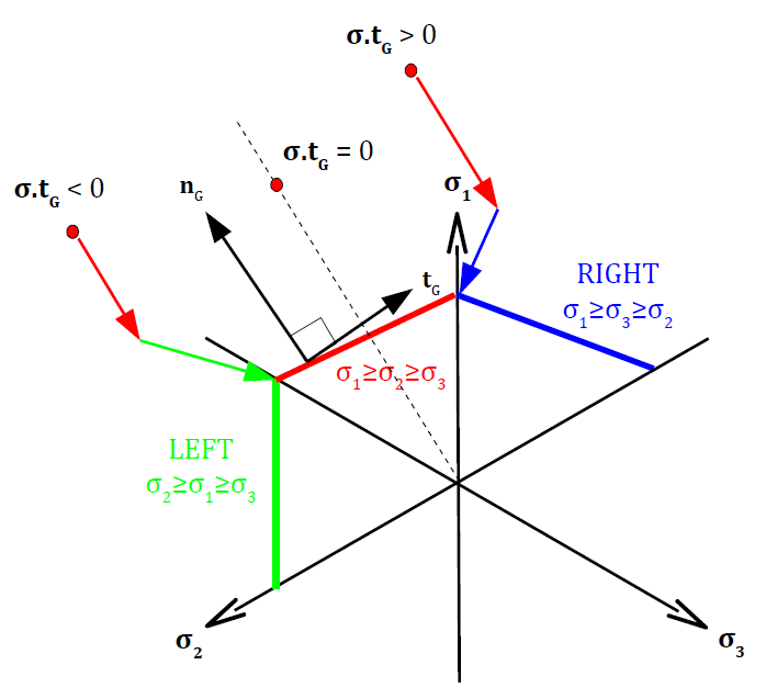
Figure 3.2.2-1: Criteria for selecting mechanisms LEFT and RIGHT
3.3. Case of the projection at the top of the cone#
We check that \({\sigma }^{\text{+}}\) obtained from the previous step () or () always checks:
If this is not the case, then it is appropriate to perform a projection at the top of the equation cone:
We therefore impose:
In the same way, the plastic deformation rate is written as:
Either:
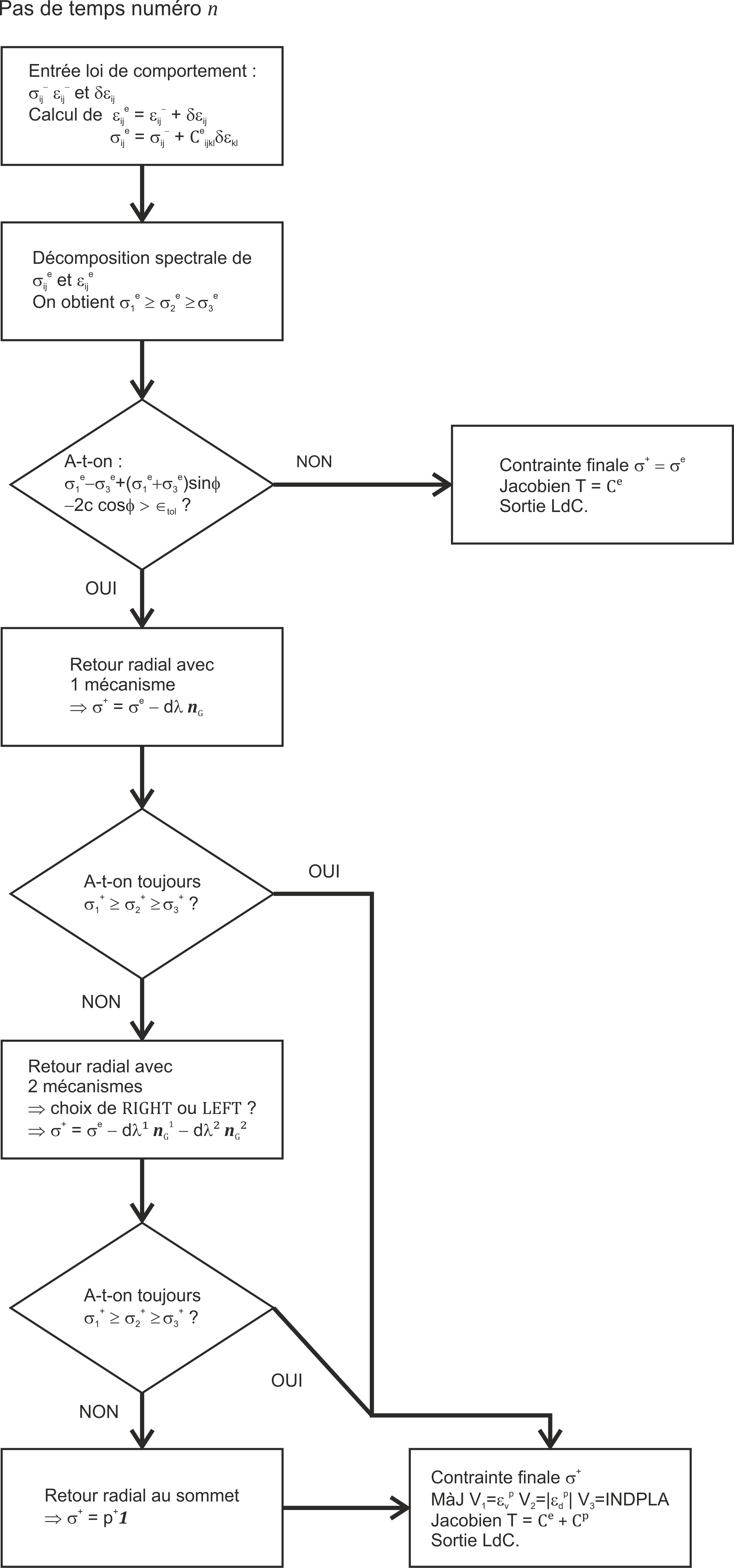
Figure 3.3-1: Mohr-Coulomb law resolution synoptic