4. Code_Aster integration#

The integration of the LETK model can be carried out according to two distinct integration schemes. The first integration schema (« historical ») is described as SPECIFIQUE and corresponds to an explicit integration schema. The second schema is built on the basis of the implicit integration schemes. It can be accessed under the keyword NEWTON_PERT.

4.1. Internal variables#

\({V}_{1}\): elastoplastic work hardening variable \({\xi }_{p}\)

\({V}_{2}\): plastic deviatoric deformation \({\gamma }_{p}\)

\({V}_{3}\): viscoplastic work hardening variable \({\xi }_{\text{vp}}\)

\({V}_{4}\): viscoplastic deviatoric deformation \({\gamma }_{\text{vp}}\)

\({V}_{5}\): \(0\) if contracture, \(1\) if dilatance

\({V}_{6}\): viscoplasticity indicator

\({V}_{7}\): plasticity indicator

\({V}_{8}\): The domains of rock behavior in plasticity

Five behavior domains, numbered from 0 to 4 (cf. figure), are identified to allow a relatively simple representation of the state of damage of the rock, from intact rock to rock in residual state. These domains are a function of the cumulative plastic deviatory deformation \({\gamma }^{p}\) and the stress state. Each domain number increment defines the transition to a higher damage domain.

If the deviator is less than 70% of the peak deviator, then the material is in the 0 range;
If not:
If \({\gamma }^{p}=0\) then the material is in domain 1;

If \(0<{\gamma }^{p}<{\gamma }^{e}\) then the material is in domain 2;

If \({\gamma }_{e}<{\gamma }^{p}<{\gamma }_{\text{ult}}\) then the material is in domain 3;

If \({\gamma }^{p}>{\gamma }_{\text{ult}}\) then the material is in domain 4.

\({V}_{9}\): position of the stress state in relation to the viscosity thresholds.

_images/10000000000002E000000411877D1B249B0E3AF5.tif

Four behavior domains, numbered from 1 to 4 (cf. figure), are identified to allow a simple representation of the viscous behavior of the material, from intact rock to rock in residual state. These domains are a function of the cumulative visco-plastic deviatory deformation \({\gamma }^{\mathit{vp}}\) and the stress state.

4.2. Explicit integration diagram (SPECIFIQUE)#

4.2.1. Update constraints#

We express the constraints updated at time + compared to those calculated at time -:

\(\sigma \mathrm{=}{\sigma }^{\mathrm{-}}+{D}^{e}{\mathit{\Delta \epsilon }}^{e}\); \(s\mathrm{=}{s}^{\mathrm{-}}+\mathrm{2G\Delta }{\tilde{\epsilon }}^{e}\); \({I}_{1}\mathrm{=}{I}_{1}^{\mathrm{-}}+{\mathrm{3K\Delta \epsilon }}_{v}^{e}\)

\({\sigma }_{\text{ij}}\mathrm{=}{s}_{\text{ij}}+\frac{{I}_{1}}{3}{\delta }_{\text{ij}}\); \({\mathit{\Delta \epsilon }}_{\text{ij}}\mathrm{=}\Delta {\tilde{\epsilon }}_{\text{ij}}+\frac{\text{tr}(\mathit{\Delta \epsilon })}{3}{\delta }_{\text{ij}}\mathrm{=}\Delta {\tilde{\epsilon }}_{\text{ij}}+\frac{{\mathit{\Delta \epsilon }}_{v}}{3}{\delta }_{\text{ij}}\); \({I}_{1}\mathrm{=}\text{tr}(\sigma )\); \({\epsilon }_{v}\mathrm{=}\text{tr}(\mathit{\Delta \epsilon })\)

Elastic prediction:

\({\sigma }^{e}\mathrm{=}{\sigma }^{\mathrm{-}}+{D}^{e}\mathit{\Delta \epsilon }\); \({s}^{e}\mathrm{=}{s}^{\mathrm{-}}+\mathrm{2G\Delta }\tilde{\epsilon }\); \({I}_{1}^{e}\mathrm{=}{I}_{1}^{\mathrm{-}}+{\mathrm{3K\Delta \epsilon }}_{v}\)

\(K\mathrm{=}{K}_{0}^{e}{\left[\frac{{I}_{1}^{\mathrm{-}}}{{\mathrm{3P}}_{a}}\right]}^{{n}_{\text{elas}}}\) and \(G\mathrm{=}{G}_{0}^{e}{\left[\frac{{I}_{1}^{\mathrm{-}}}{{\mathrm{3P}}_{a}}\right]}^{{n}_{\text{elas}}}\)

Note: The compression coefficient \(K\) and the shear modulus \(G\) are considered at the moment -.

4.2.1.1. Hypoelasticity#

\({\mathit{\Delta \sigma }}_{\text{ij}}\mathrm{=}{\mathit{\Delta s}}_{\text{ij}}+\frac{{\mathit{\Delta I}}_{1}}{3}{\delta }_{\text{ij}}\) \({\mathit{\Delta \epsilon }}_{\text{ij}}\mathrm{=}\Delta {\tilde{\epsilon }}_{\text{ij}}+\frac{{\mathit{\Delta \epsilon }}_{v}}{3}{\delta }_{\text{ij}}\) \({\mathit{\Delta \sigma }}_{\text{ij}}\mathrm{=}{\mathrm{2G\Delta \epsilon }}_{\text{ij}}+(K\mathrm{-}\frac{\mathrm{2G}}{3})\text{tr}(\mathit{\Delta \epsilon }){\delta }_{\text{ij}}\)

\(\left\{\begin{array}{c}\Delta {\sigma }_{\text{11}}\\ \Delta {\sigma }_{\text{22}}\\ \Delta {\sigma }_{\text{33}}\\ \sqrt{2}\Delta {\sigma }_{\text{12}}\\ \sqrt{2}\Delta {\sigma }_{\text{13}}\\ \sqrt{2}\Delta {\sigma }_{\text{23}}\end{array}\right\}\mathrm{=}\underset{{D}^{e}}{\underset{\underbrace{}}{\left[\begin{array}{cccccc}\frac{\mathrm{4G}}{3}+K& K\mathrm{-}\frac{\mathrm{2G}}{3}& K\mathrm{-}\frac{\mathrm{2G}}{3}& 0& 0& 0\\ K\mathrm{-}\frac{\mathrm{2G}}{3}& \frac{\mathrm{4G}}{3}+K& K\mathrm{-}\frac{\mathrm{2G}}{3}& 0& 0& 0\\ K\mathrm{-}\frac{\mathrm{2G}}{3}& K\mathrm{-}\frac{\mathrm{2G}}{3}& \frac{\mathrm{4G}}{3}+K& 0& 0& 0\\ 0& 0& 0& \mathrm{2G}& 0& 0\\ 0& 0& 0& 0& \mathrm{2G}& 0\\ 0& 0& 0& 0& 0& \mathrm{2G}\end{array}\right]}}\text{.}\left\{\begin{array}{c}{\mathit{\Delta \epsilon }}_{\text{11}}\\ \Delta {\varepsilon }_{\text{22}}\\ \Delta {\varepsilon }_{\text{33}}\\ \sqrt{2}\Delta {\varepsilon }_{\text{12}}\\ \sqrt{2}\Delta {\varepsilon }_{\text{13}}\\ \sqrt{2}\Delta {\varepsilon }_{\text{23}}\end{array}\right\}\)

4.2.1.2. Plasticity and viscoplasticity#

We express the constraint field at time \(+\):

\({\sigma }_{\text{ij}}={\sigma }_{\text{ij}}^{-}+{D}_{\text{ijkl}}^{e}{\mathrm{\Delta \epsilon }}_{\text{kl}}^{e}={\sigma }_{\text{ij}}^{-}+{D}_{\text{ijkl}}^{e}({\mathrm{\Delta \epsilon }}_{\text{kl}}-{\mathrm{\Delta \epsilon }}_{\text{kl}}^{p}-{\mathrm{\Delta \epsilon }}_{\text{kl}}^{\text{vp}})\)

Which is written by replacing the increase in plastic and viscous deformations by their expressions in the form:

\({\sigma }_{\text{ij}}={\sigma }_{\text{ij}}^{-}+{D}_{\text{ijkl}}^{e}({\mathrm{\Delta \epsilon }}_{\text{kl}}-{\mathrm{\Delta \lambda G}}_{\text{kl}}({\sigma }^{-},{\xi }_{p}^{-})-\langle \phi \rangle {G}_{\text{kl}}^{\text{visc}}({\sigma }^{-},{\xi }_{v}^{-})\mathrm{\Delta t})\)

The main unknown is the plastic multiplier \(\mathrm{\Delta \lambda }\).

We’re looking for \(\mathit{\Delta \lambda }\mathrm{/}{f}^{d}(\sigma ,{\xi }_{p})\mathrm{=}0\)

\({f}^{d}({\sigma }_{\text{ij}}^{-}+{D}_{\text{ijkl}}^{e}({\mathrm{\Delta \epsilon }}_{\text{kl}}-{\mathrm{\Delta \lambda G}}_{\text{kl}}({\sigma }^{-},{\xi }_{p}^{-})-\langle \phi \rangle {G}_{\text{kl}}^{\text{visc}}({\sigma }^{-},{\xi }_{v}^{-})\mathrm{\Delta t}),{\xi }_{p}^{-}+{\mathrm{\Delta \xi }}_{p})=0\)

with \({\mathit{\Delta \gamma }}_{p}\mathrm{=}\mathit{\Delta \lambda }\sqrt{\frac{2}{3}{\tilde{G}}_{\text{ij}}{\tilde{G}}_{\text{ij}}}\mathrm{=}\mathit{\Delta \lambda }\sqrt{\frac{2}{3}}{G}_{\text{II}}\)

We choose to make an explicit resolution with an Euler expansion:

\({f}^{d}({\sigma }_{\text{ij}}^{-}+{D}_{\text{ijkl}}^{e}{\mathrm{\Delta \epsilon }}_{\text{kl}}-{D}_{\text{ijkl}}^{e}\langle \Phi \rangle {G}_{\text{kl}}^{\text{visc}}({\sigma }^{-},{\xi }_{v}^{-})\mathrm{\Delta t},{\xi }_{p}^{-})-\frac{\partial {f}^{d}}{\partial {\sigma }_{\text{ij}}}{D}_{\text{ijkl}}^{e}{G}_{\text{kl}}({\sigma }^{-},{\xi }_{p}^{-})\mathrm{\Delta \lambda }+\frac{\partial {f}^{d}}{\partial {\xi }_{p}}{\mathrm{\Delta \xi }}_{p}=0\)

A distinction is made between the two cases:

\({\mathrm{\Delta \xi }}_{p}={\mathrm{\Delta \gamma }}_{p}+{\mathrm{\Delta \gamma }}_{\text{vp}}\) (dilating case: the stress state exceeds the contract/dilatance limit)

\({f}^{d}({\sigma }_{\text{ij}}^{\mathrm{-}}+{D}_{\text{ijkl}}^{e}{\mathit{\Delta \epsilon }}_{\text{kl}}\mathrm{-}{D}_{\text{ijkl}}^{e}\mathrm{\langle }\Phi \mathrm{\rangle }{G}_{\text{kl}}^{\text{visc}}({\sigma }^{\mathrm{-}},{\xi }_{v}^{\mathrm{-}})\mathit{\Delta t},{\xi }_{p}^{\mathrm{-}})\)

\(\mathrm{-}\frac{\mathrm{\partial }{f}^{d}}{\mathrm{\partial }{\sigma }_{\text{ij}}}{D}_{\text{ijkl}}^{e}{G}_{\text{kl}}({\sigma }^{\mathrm{-}},{\xi }_{p}^{\mathrm{-}})\mathit{\Delta \lambda }+\frac{\mathrm{\partial }{f}^{d}}{\mathrm{\partial }{\xi }_{p}}({\mathit{\Delta \gamma }}_{p}+{\mathit{\Delta \gamma }}_{\text{vp}})\mathrm{=}0\)

\(\begin{array}{c}{f}^{d}({\sigma }_{\mathit{ij}}^{\mathrm{-}}+{D}_{\mathit{ijkl}}^{e}\Delta {\epsilon }_{\mathit{kl}}\mathrm{-}{D}_{\mathit{ijkl}}^{e}<\Phi >{G}_{\mathit{kl}}^{\mathit{visc}}({\sigma }^{\mathrm{-}},{\xi }_{v}^{\mathrm{-}})\Delta t,{\xi }_{p}^{\mathrm{-}})\mathrm{=}\\ (\frac{\mathrm{\partial }{f}^{d}}{\mathrm{\partial }{\sigma }_{\mathit{ij}}}{D}_{\mathit{ijkl}}^{e}{G}_{\mathit{kl}}({\sigma }^{\mathrm{-}},{\xi }_{p}^{\mathrm{-}})\mathrm{-}\frac{\mathrm{\partial }{f}^{d}}{\mathrm{\partial }{\xi }_{p}}\sqrt{\frac{2}{3}}{G}_{\mathit{II}}({\sigma }^{\mathrm{-}},{\xi }_{p}^{\mathrm{-}})\Delta \lambda \mathrm{-}\frac{\mathrm{\partial }{f}^{d}}{\mathrm{\partial }{\xi }_{p}}\Delta {\gamma }_{\mathit{vp}})\end{array}\)

\(\mathrm{\Delta \lambda }=\frac{{f}^{d}({\sigma }_{\text{ij}}^{-},{\xi }_{p}^{-})+\frac{\partial {f}^{d}}{\partial {\xi }_{p}}{\mathrm{\Delta \gamma }}_{\text{vp}}+\frac{\partial {f}^{d}}{\partial {\sigma }_{\text{ij}}}\left[{D}_{\text{ijkl}}^{e}{\mathrm{\Delta \epsilon }}_{\text{kl}}-{D}_{\text{ijkl}}^{e}\langle \Phi \rangle {G}_{\text{kl}}^{\text{visc}}({\sigma }^{-},{\xi }_{\text{vp}}^{-})\mathrm{\Delta t}\right]}{(\frac{\partial {f}^{d}}{\partial {\sigma }_{\text{ij}}}{D}_{\text{ijkl}}^{e}{G}_{\text{kl}}({\sigma }^{-},{\xi }_{p}^{-})-\frac{\partial {f}^{d}}{\partial {\xi }_{p}}\sqrt{\frac{2}{3}}{\tilde{G}}_{\text{II}}({\sigma }^{-},{\xi }_{p}^{-}))}\)

\({\mathrm{\Delta \xi }}_{p}={\mathrm{\Delta \gamma }}_{p}\) (contracting case: the stress state is below the contract/dilatance limit)

\(\mathrm{\Delta \lambda }=\frac{{f}^{d}({\sigma }_{\text{ij}}^{-},{\xi }_{p}^{-})+\frac{\partial {f}^{d}}{\partial {\sigma }_{\text{ij}}}\left[{D}_{\text{ijkl}}^{e}{\mathrm{\Delta \epsilon }}_{\text{kl}}-{D}_{\text{ijkl}}^{e}\langle \Phi \rangle {G}_{\text{kl}}^{\text{visc}}({\sigma }^{-},{\xi }_{\text{vp}}^{-})\mathrm{\Delta t}\right]}{(\frac{\partial {f}^{d}}{\partial {\sigma }_{\text{ij}}}{D}_{\text{ijkl}}^{e}{G}_{\text{kl}}({\sigma }^{-},{\xi }_{p}^{-})-\frac{\partial {f}^{d}}{\partial {\xi }_{p}}\sqrt{\frac{2}{3}}{\tilde{G}}_{\text{II}}({\sigma }^{-},{\xi }_{p}^{-}))}\)

with \(\Phi ={A}_{v}{(\frac{{f}^{\text{vp}}({\sigma }^{e},{\xi }_{\text{vp}}^{-})}{\text{Pa}})}^{{n}_{v}}\), \({A}_{v}\), and \({n}_{v}\) are model parameters.

4.2.2. Tangent operator#

The constraint in state \(+\):

\(\begin{array}{}{\sigma }_{\mathrm{ij}}={\sigma }_{\mathrm{ij}}^{-}+{D}_{\mathrm{ijkl}}^{e}\Delta {\epsilon }_{\mathrm{kl}}^{e}={\sigma }_{\mathrm{ij}}^{-}+{D}_{\mathrm{ijkl}}^{e}(\Delta {\epsilon }_{\mathrm{kl}}-\Delta {\epsilon }_{\mathrm{kl}}^{p}-\Delta {\epsilon }_{\mathrm{kl}}^{\mathrm{vp}})=\\ {\sigma }_{\mathrm{ij}}^{-}+{D}_{\mathrm{ijkl}}^{e}(\Delta {\epsilon }_{\mathrm{kl}}-\Delta \lambda {G}_{\mathrm{kl}}({\sigma }^{-},{\xi }_{p}^{-})-\langle \Phi \rangle {G}_{\mathrm{kl}}^{\mathrm{visc}}({\sigma }^{-},{\xi }_{\mathrm{vp}}^{-})\Delta t)\end{array}\)

\(\frac{\partial {\sigma }_{\text{ij}}}{\partial {\mathrm{\Delta \epsilon }}_{\text{kl}}}={D}_{\text{ijkl}}^{e}-{D}_{\text{ijmn}}^{e}{G}_{\text{mn}}^{-}\frac{\partial \mathrm{\Delta \lambda }}{\partial {\mathrm{\Delta \epsilon }}_{\text{kl}}}-{D}_{\text{ijmn}}^{e}{G}_{\text{imn}}^{\text{visc}-}\frac{\partial \langle \phi \rangle }{\partial {\mathrm{\Delta \epsilon }}_{\text{kl}}}\mathrm{\Delta t}\)

A distinction is made between the two cases:

\({\mathrm{\Delta \xi }}_{p}={\mathrm{\Delta \gamma }}_{p}\) (contracting case: the state of constraints is below the characteristic threshold)

\(\mathrm{\Delta \lambda }=\frac{{f}^{d}({\sigma }_{\text{ij}}^{-},{\xi }_{p}^{-})+\frac{\partial {f}^{d}}{\partial {\sigma }_{\text{ij}}}\left[{D}_{\text{ijkl}}^{e}{\mathrm{\Delta \epsilon }}_{\text{kl}}-{D}_{\text{ijkl}}^{e}\langle \Phi \rangle {G}_{\text{kl}}^{\text{visc}}({\sigma }^{-},{\xi }_{v}^{-})\mathrm{\Delta t}\right]}{(\frac{\partial {f}^{d}}{\partial {\sigma }_{\text{ij}}}{D}_{\text{ijkl}}^{e}{G}_{\text{kl}}({\sigma }^{-},{\xi }_{p}^{-})-\frac{\partial {f}^{d}}{\partial {\xi }_{p}}\sqrt{\frac{2}{3}}{\tilde{G}}_{\text{II}}({\sigma }^{-},{\xi }_{p}^{-}))}\) and \(\Phi ={A}_{v}{(\frac{{f}^{\text{vp}}({\sigma }^{e},{\xi }_{\text{vp}}^{-})}{\text{Pa}})}^{{n}_{v}}\)

\(\frac{\partial \Phi }{\partial {\mathrm{\Delta \epsilon }}_{\text{kl}}}=\frac{{A}_{v}\text{.}{n}_{v}}{\text{Patm}}{(\frac{{f}^{\text{vp}}({\sigma }^{e},{\xi }_{\text{vp}}^{-})}{\text{Patm}})}^{{n}_{v}-1}\text{.}\frac{\partial {f}^{\text{vp}}}{\partial {\sigma }_{\text{ij}}^{e}}\text{.}\frac{\partial {\sigma }_{\text{ij}}^{e}}{\partial {\mathrm{\Delta \epsilon }}_{\text{kl}}}=\frac{{A}_{v}\text{.}{n}_{v}}{\text{Patm}}{(\frac{{f}^{\text{vp}}({\sigma }^{e},{\xi }_{\text{vp}}^{-})}{\text{Patm}})}^{{n}_{v}-1}\text{.}\frac{\partial {f}^{\text{vp}}}{\partial {\sigma }_{\text{ij}}^{e}}\text{.}{D}_{\text{ijkl}}^{e}\)

\(\begin{array}{}\frac{\partial {\sigma }_{\text{ij}}}{\partial {\mathrm{\Delta \epsilon }}_{\text{kl}}}={D}_{\text{ijkl}}^{e}-{D}_{\text{ijmn}}^{e}\text{.}{G}_{\text{mn}}^{-}\frac{\frac{\partial {f}^{d}}{\partial {\sigma }_{\text{ij}}}\text{.}\left[{D}_{\text{ijkl}}^{e}-{D}_{\text{ijmn}}^{e}{G}_{\text{mn}}^{\text{visc}}({\sigma }^{-},{\xi }_{p}^{-})\frac{\partial \Phi }{\partial {\mathrm{\Delta \epsilon }}_{\text{kl}}}\mathrm{\Delta t}\right]}{(\frac{\partial {f}^{d}}{\partial {\sigma }_{\text{ij}}}{D}_{\text{ijkl}}^{e}{G}_{\text{kl}}({\sigma }^{-},{\xi }_{p}^{-})-\frac{\partial {f}^{d}}{\partial {\xi }_{p}}\sqrt{\frac{2}{3}}{\tilde{G}}_{\text{II}}({\sigma }^{-},{\xi }_{p}^{-}))}-\\ {D}_{\text{ijmn}}^{e}\text{.}{G}_{\text{mn}}^{\text{visc}-}\frac{{A}_{v}\text{.}{n}_{v}}{\text{Patm}}{(\frac{{f}^{\text{vp}}({\sigma }^{e},{\xi }_{\text{vp}}^{-})}{\text{Patm}})}^{{n}_{v}-1}\text{.}\frac{\partial {f}^{\text{vp}}}{\partial {\sigma }_{\text{ij}}^{e}}\text{.}{D}_{\text{ijkl}}^{e}\mathrm{\Delta t}\end{array}\)

\(\Delta {\xi }_{p}\mathrm{=}\Delta {\gamma }_{p}+\Delta {\gamma }_{v}\) (dilating case: the stress state exceeds the characteristic threshold)

\(\frac{\partial \mathrm{\Delta \lambda }}{\partial {\mathrm{\Delta \epsilon }}_{\text{kl}}}=\frac{\frac{\partial {f}^{d}}{\partial {\sigma }_{\text{ij}}}\text{.}\left[{D}_{\text{ijkl}}^{e}-{D}_{\text{ijmn}}^{e}{G}_{\text{mn}}^{\text{visc}}({\sigma }^{-},{\xi }_{p}^{-})\frac{\partial \Phi }{\partial {\mathrm{\Delta \epsilon }}_{\text{kl}}}\mathrm{\Delta t}\right]+\frac{\partial {f}^{d}}{\partial {\xi }_{p}}\text{.}\frac{\partial {\mathrm{\Delta \gamma }}_{\text{vp}}}{\partial {\mathrm{\Delta \epsilon }}_{\text{kl}}^{\text{vp}}}\text{.}\frac{\partial {\mathrm{\Delta \epsilon }}_{\text{kl}}^{\text{vp}}}{\partial {\mathrm{\Delta \sigma }}_{\text{ij}}^{e}}\text{.}{D}_{\text{ijkl}}^{e}}{(\frac{\partial {f}^{d}}{\partial {\sigma }_{\text{ij}}}{D}_{\text{ijmn}}^{e}{G}_{\text{mn}}({\sigma }^{-},{\xi }_{p}^{-})-\frac{\partial {f}^{d}}{\partial {\xi }_{p}}\sqrt{\frac{2}{3}}{\tilde{G}}_{\text{II}}({\sigma }^{-},{\xi }_{p}^{-}))}\)

where:

\(\frac{\partial {\mathrm{\Delta \gamma }}_{\text{vp}}}{\partial {\mathrm{\Delta \epsilon }}_{\text{kl}}^{\text{vp}}}=\frac{1}{2}{(\frac{2}{3}\Delta {\tilde{\epsilon }}_{\text{ij}}^{\text{vp}}\text{.}\Delta {\tilde{\epsilon }}_{\text{ij}}^{\text{vp}})}^{-\frac{1}{2}}\text{.}\frac{2}{3}\text{.}2\text{.}\Delta {\tilde{\epsilon }}_{\text{ij}}^{\text{vp}}\text{.}\frac{\partial \Delta {\tilde{\epsilon }}_{\text{ij}}^{\text{vp}}}{\partial {\mathrm{\Delta \epsilon }}_{\text{kl}}^{\text{vp}}}=\frac{2}{3}\text{.}\frac{\Delta {\tilde{\epsilon }}_{\text{ij}}^{\text{vp}}}{{\mathrm{\Delta \gamma }}_{\text{vp}}}\text{.}({\delta }_{\text{ik}}\text{.}{\delta }_{\text{jl}}-\frac{1}{3}{\delta }_{\text{ij}}\text{.}{\delta }_{\text{kl}})\)

\(\frac{\partial {\mathrm{\Delta \epsilon }}_{\text{kl}}^{\text{vp}}}{\partial {\mathrm{\Delta \sigma }}_{\text{ij}}^{e}}=\frac{{n}_{v}\text{.}{A}_{v}}{\text{Patm}}\text{.}{(\frac{{f}^{\text{vp}}({\sigma }^{e},{\xi }_{v}^{-})}{\text{Patm}})}^{{n}_{v}-1}\text{.}\frac{\partial {f}^{\text{vp}}}{\partial {\sigma }_{\text{ij}}^{e}}\text{.}{G}_{\text{kl}}^{\text{visc}-}({\sigma }^{-},{\xi }_{\text{vp}}^{-})\mathrm{\Delta t}\)

4.2.3. Resolution algorithm in Code_Aster#

Change in the sign of the stresses in state \(\mathrm{-}\) and the increase in deformation:

\({\sigma }_{L\wedge K}^{-}=-{\sigma }^{-}\)

\({\mathrm{\Delta \epsilon }}_{L\wedge K}=-\mathrm{\Delta \epsilon }\)

Calculation of the elastic prediction constraint \({\sigma }^{e}\): \({\sigma }^{e}={\sigma }^{-}+{D}^{e}\mathrm{\Delta \epsilon }\)
Verification of the sign of the viscous criterion with the viscous variable max: \({f}^{\text{vp}}({\sigma }^{e},{\xi }_{\text{vp}-\text{max}})\)
If \({f}^{\text{vp}}({\sigma }^{e},{\xi }_{\text{vp}-\text{max}})>0\): expansion case and combined work hardening \({V}_{5}=1\). The combination between the plastic work hardening variable and the viscous variable is considered to be the work-hardening variable of the plastic criterion: \(\Delta {\xi }_{p}\mathrm{=}\Delta {\gamma }_{p}+\Delta {\gamma }_{\text{vp}}\)
If \({f}^{\text{vp}}({\sigma }^{e},{\xi }_{\text{vp}-\text{max}})<0\): contracting case and uncoupled work hardening \({V}_{5}\mathrm{=}0\). The work-hardening variable for the plastic criterion is the plastic variable: \(\Delta {\xi }_{p}\mathrm{=}\Delta {\gamma }_{p}\)

For the viscous criterion: \({u}^{\text{vp}}={A}^{\text{vp}}({\xi }_{\text{vp}}){s}_{\text{II}}H(\theta )+{B}^{\text{vp}}({\xi }_{\text{vp}}){I}_{1}+{D}^{\text{vp}}({\xi }_{\text{vp}})\)

If \({u}^{\text{vp}}({\sigma }^{e},{\xi }_{\text{vp}}^{-})<0\):

if \(-\frac{{D}^{\text{vp}}}{{B}^{\text{vp}}}<-\frac{{D}^{d}}{{B}^{d}}\) (Figure 4.2.3-a) then redistricting the time step

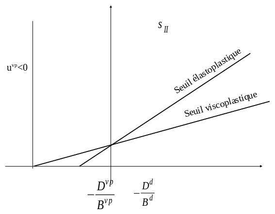
Figure 4.2.3-a *. Schematic representation in the case*\({u}^{\text{vp}}({\sigma }^{e},{\xi }_{\text{vp}}^{-})<0`**, ** :math:\)-frac{{D}^{text{vp}}}{{B}^{text{vp}}}<-frac{{D}^{d}}{{B}^{d}}`

Otherwise (Figure 4.2.3-b) two cases occur:

if \({\sigma }^{e}\) is in zone \(A\) then \({f}^{\text{vp}}({\sigma }^{e})\) is not defined but we can make a geometric projection (cf. note in paragraph 3.3.3)
if \({\sigma }^{e}\) is in zone \(B\) then you have to make a projection to the top.

We are then satisfied with the message: « Stop for non-coherent material coefficients of the law ».

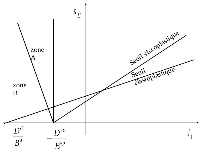
Figure 4.2.3-b.Schematic representation in case \({u}^{\text{vp}}({\sigma }^{e},{\xi }_{\text{vp}}^{-})<0\), \(-\frac{{D}^{d}}{{B}^{d}}<-\frac{{D}^{\text{vp}}}{{B}^{\text{vp}}}\)

For the elastoplastic criterion:

\({u}^{d}={A}^{d}({\xi }_{p}){s}_{\text{II}}H(\theta )+{B}^{d}({\xi }_{p}){I}_{1}+{D}^{d}({\xi }_{p})\)

If \({u}^{d}({\sigma }^{e},{\xi }_{p}^{-})<0\) then there is a redistribution of the time step

For the viscous criterion:

If \({f}^{\text{vp}}({\sigma }^{e},{\xi }_{\text{vp}}^{-})<0\) then no creep and \({\mathrm{\Delta \epsilon }}_{\text{vp}}=0\)

If \({f}^{\text{vp}}({\sigma }^{e},{\xi }_{\text{vp}}^{-})>0\) then creep develops in the following form:

\({\mathrm{\Delta \epsilon }}_{\text{vp}}=A{\left[\frac{\langle {f}^{\text{vp}}({\sigma }^{e},{\xi }_{\text{vp}}^{-})\rangle }{\text{Patm}}\right]}^{{n}_{v}}{G}^{\text{visc}}({\sigma }^{-},{\xi }_{\text{vp}}^{-})\mathrm{\Delta t}\) with \({G}^{\text{visc}}=\frac{\partial {f}^{\text{vp}}}{\partial \sigma }-(\frac{\partial {f}^{\text{vp}}}{\partial \sigma }n)n\)

\(\langle \rangle\): Macauley’s hooks

where \(\text{sin}(\Psi )\mathrm{=}{\mu }_{\mathrm{0,}v}(\frac{{\sigma }_{\text{max}}\mathrm{-}{\sigma }_{\text{lim}}}{{\xi }_{\mathrm{0,}v}{\sigma }_{\text{max}}+{\sigma }_{\text{lim}}})\) (see § 3.6.1), \({\beta }^{\text{'}}\), and \(n\) are deduced

we can deduce \(\Delta {\gamma }_{\text{vp}}\mathrm{=}\sqrt{\frac{2}{3}\Delta {\tilde{\varepsilon }}_{\text{vp}}\text{.}\Delta {\tilde{\varepsilon }}_{\text{vp}}}>0\) where \(\Delta {\tilde{\varepsilon }}_{\text{vp}}\mathrm{=}\Delta {\varepsilon }_{\text{vp}}\mathrm{-}\frac{\text{tr}(\Delta {\varepsilon }_{\text{vp}})}{3}{I}^{d}\)

update of the work-hardening variable for the viscous criterion:

\({\xi }_{\text{vp}}\mathrm{=}{\xi }_{\text{vp}}^{\mathrm{-}}+\Delta {\xi }_{\text{vp}}\) with \(\Delta {\xi }_{\text{vp}}\mathrm{=}\text{Min}\left[\Delta {\gamma }_{\text{vp}},{\xi }_{v\mathrm{-}\text{max}}\mathrm{-}{\xi }_{\text{vp}}^{\mathrm{-}}\right]\)

updating the constraints: \(\sigma ={\sigma }^{e}-{D}^{e}{\mathrm{\Delta \epsilon }}_{\text{vp}}\)

updating the internal variables:

\({V}_{1}={\xi }_{p}={\xi }_{p}^{-}+{\mathrm{\Delta \gamma }}_{\text{vp}}\)

\({V}_{2}={\gamma }_{p}={\gamma }_{p}^{-}\)

\({V}_{3}={\xi }_{\text{vp}}={\xi }_{\text{vp}}^{-}+{\mathrm{\Delta \xi }}_{\text{vp}}\)

\({V}_{4}={\gamma }_{\text{vp}}={\gamma }_{\text{vp}}^{-}+{\mathrm{\Delta \gamma }}_{\text{vp}}\)

For the elastoplastic criterion:

If \({f}^{d}({\sigma }^{e}\mathrm{-}{D}^{e}{\mathit{\Delta \xi }}_{\text{vp}},{\xi }_{p}^{\mathrm{-}}+\Delta {\gamma }_{\text{vp}})\mathrm{\le }0\) then: \(\Delta \gamma \mathrm{=}\Delta {\gamma }_{p}\mathrm{=}\Delta {\xi }_{p}\mathrm{=}0\)
If \({f}^{d}({\sigma }^{e}\mathrm{-}{D}^{e}{\mathit{\Delta \epsilon }}_{\text{vp}},{\xi }_{p}^{\mathrm{-}}+\Delta {\gamma }_{\text{vp}})>0\) then: \(\Delta {\tilde{\epsilon }}_{p}=\mathrm{\Delta \lambda G}({\sigma }^{-},{\xi }_{p}^{-})\) with

\(\text{sin}(\Psi )={\mu }_{\mathrm{0,}v}(\frac{{\sigma }_{\text{max}}-{\sigma }_{\text{lim}}}{{\xi }_{\mathrm{0,}v}{\sigma }_{\text{max}}+{\sigma }_{\text{lim}}})\) (see § 3.6.1) if \(0\mathrm{\le }{\xi }_{p}^{\mathrm{-}}<{\xi }_{\text{pic}}\)

\(\text{sin}(\Psi )={\mu }_{1}(\frac{\alpha -{\alpha }_{\text{res}}}{{\xi }_{1}\alpha -{\alpha }_{\text{res}}})\) (see § 3.6.2) if \({\xi }_{p}^{-}>{\xi }_{\text{pic}}\)

\(G=\frac{\partial {f}^{d}}{\partial \sigma }-(\frac{\partial {f}^{d}}{\partial \sigma }n)n\) \({\beta }^{\text{'}}\) and \(n\) are deducted

We’re looking for \(\mathrm{\Delta \lambda }>0\) such as \({f}^{d}(\sigma ,{\xi }_{p}^{-})=0\)

We deduce \(\Delta {\gamma }_{p}>0\)

If uncoupled work hardening (contracting) \({f}^{d}({\sigma }^{e}-{D}^{e}{\mathrm{\Delta \xi }}_{\text{vp}},{\xi }_{p}^{-}+{\mathrm{\Delta \gamma }}_{\text{vp}})\le 0\) then: \(\Delta {\xi }_{p}\mathrm{=}\Delta {\gamma }_{p}\)

if not coupled work hardening (dilatance) \({f}^{d}({\sigma }^{e}\mathrm{-}{D}^{e}{\mathit{\Delta \epsilon }}_{\text{vp}},{\xi }_{p}^{\mathrm{-}}+\Delta {\gamma }_{\text{vp}})>0\) then: \(\Delta {\xi }_{p}\mathrm{=}\Delta {\gamma }_{p}+\Delta {\gamma }_{\text{vp}}\)

The table of internal variables is completed:

\({V}_{1}={\xi }_{p}={\xi }_{p}^{-}+{\mathrm{\Delta \xi }}_{p}\)

\({V}_{2}={\gamma }_{p}={\gamma }_{p}^{-}+{\mathrm{\Delta \gamma }}_{p}\)

Constraints update:

\({\mathrm{\Delta \epsilon }}^{\text{irr}}={\mathrm{\Delta \epsilon }}^{\text{vp}}+{\mathrm{\Delta \epsilon }}^{p}\)

\({\mathrm{\Delta \epsilon }}^{e}=\mathrm{\Delta \epsilon }-{\mathrm{\Delta \epsilon }}^{\text{irr}}\)

\(\mathrm{\Delta \sigma }={D}^{e}{\mathrm{\Delta \epsilon }}^{e}\)

\(\sigma ={\sigma }^{-}+\mathrm{\Delta \sigma }\)

Algorithm Summary

\({\sigma }^{e}\mathrm{=}{\sigma }^{\mathrm{-}}+{D}^{e}\mathit{\Delta \epsilon }\)
if \({f}^{\text{vp}}({\sigma }^{e},{\xi }_{v\text{max}})<0\) then contractance (\(\mathit{VARV}\mathrm{=}0\)) and the plastic variable is \(\Delta {\xi }^{p}\mathrm{=}\Delta {\gamma }^{p}\)
if \({f}^{\text{vp}}({\sigma }^{e},{\xi }_{v\text{max}})>0\) then dilatance (\(\mathit{VARV}\mathrm{=}1\)) and the plastic variable is \({\mathrm{\Delta \xi }}^{p}={\mathrm{\Delta \gamma }}^{p}+{\mathrm{\Delta \gamma }}^{\text{vp}}\)

Creep check: * calculation of \({f}^{\text{vp}}({\sigma }^{e},{\xi }_{\text{vp}}^{-})\) if :math:`{f}^{text{vp}}({sigma }^{e},{xi }_{text{vp}}^{-})<0` (**No creep) * \(\Delta {\xi }_{\text{vp}}\mathrm{=}\Delta {\gamma }_{\text{vp}}\mathrm{=}0\) \({\xi }_{\text{vp}}={\xi }_{\text{vp}}^{-}\) \({\gamma }_{\text{vp}}\mathrm{=}{\gamma }_{\text{vp}}^{\mathrm{-}}\) if :math:`{f}^{text{vp}}({sigma }^{e},{xi }_{text{vp}}^{mathrm{-}})>0` (**creep) * Calculate \({\mathrm{\Delta \epsilon }}_{\text{vp}}\) and \({\mathrm{\Delta \gamma }}_{\text{vp}}\) based on \({\sigma }^{e}\) and \({\xi }_{\text{vp}}^{-}\) \(\Delta {\xi }_{\text{vp}}\mathrm{=}\text{min}(\Delta {\gamma }_{\text{vp}},{\xi }_{v\mathrm{-}\text{max}}\mathrm{-}{\xi }_{\text{vp}}^{\mathrm{-}})\) \({\xi }_{\text{vp}}={\xi }_{\text{vp}}^{-}+{\mathrm{\Delta \xi }}_{\text{vp}}\) \({\gamma }_{\text{vp}}\mathrm{=}{\gamma }_{\text{vp}}^{\mathrm{-}}+\Delta {\gamma }_{\text{vp}}\) * Elastic prediction adjustment: \({\sigma }_{n}^{e}\mathrm{=}{\sigma }^{e}\mathrm{-}{D}^{e}{\mathit{\Delta \epsilon }}_{\text{vp}}\) Plasticity checking: * calculation of \({f}^{d}({\sigma }_{n}^{e},{\xi }_{p}^{\mathrm{-}}+\Delta {\gamma }_{\text{vp}})\) if :math:`{f}^{d}({sigma }_{n}^{e},{xi }_{p}^{mathrm{-}}+Delta {gamma }_{text{vp}})<0` (Elasticity*) ** \(\Delta {\varepsilon }_{p}\mathrm{=}\Delta {\gamma }_{p}\mathrm{=}0\) \({\gamma }_{p}\mathrm{=}{\gamma }_{p}^{\mathrm{-}}\) \({\xi }_{p}={\xi }_{p}^{-}+{\mathrm{\Delta \xi }}_{p}\) with \(\Delta {\xi }_{p}\mathrm{=}0\) if \(\mathit{VARV}\mathrm{=}0\) \(\Delta {\xi }_{p}\mathrm{=}\Delta {\gamma }_{\text{vp}}\) if \(\mathit{VARV}\mathrm{=}1\) constraint update: \(\sigma \mathrm{=}{\sigma }^{e}\mathrm{-}{D}^{e}{\mathit{\Delta \epsilon }}_{\text{vp}}\) if :math:`{f}^{d}({sigma }_{n}^{e},{xi }_{p}^{mathrm{-}}+Delta {gamma }_{text{vp}})>0` (**Plasticity) * Calculating \(\Delta \lambda\), \({\mathit{\Delta \gamma }}_{p}\), and \(\Delta {\varepsilon }_{p}\) \(\Delta {\xi }_{p}\mathrm{=}\Delta {\gamma }_{p}\) if \(\mathit{VARV}\mathrm{=}0\) \(\Delta {\varepsilon }_{p}\mathrm{=}\Delta {\gamma }_{p}+\Delta {\gamma }_{\text{vp}}\) if \(\mathit{VARV}\mathrm{=}1\) \({\xi }_{p}\mathrm{=}{\xi }_{p}^{\mathrm{-}}+\Delta {\xi }_{p}\) constraint update: \(\sigma \mathrm{=}{\sigma }^{\mathrm{-}}+{D}^{e}(\Delta \varepsilon \mathrm{-}\Delta {\varepsilon }_{\text{vp}}\mathrm{-}\Delta {\varepsilon }_{p})\) table of internal variables: \(\mathit{V1}\mathrm{=}{\xi }_{p}\) \(\mathit{V2}\mathrm{=}{\gamma }_{p}\) \(\mathit{V3}\mathrm{=}{\xi }_{\text{vp}}\) \(\mathit{V4}\mathrm{=}{\gamma }_{\text{vp}}\) \(\mathit{V5}\mathrm{=}\mathit{VARV}\) (0 if contracture or 1 if dilatance) \(\mathit{V6}\mathrm{=}\) viscosity indicator \(\mathit{V7}\mathrm{=}\) plasticity indicator

4.3. Implicit integration diagram#

The integration of the model LETK according to the implicit integration scheme is carried out under environment PLASTI. The integration of model LETK under an implicit schema is currently available only by calculating a disturbed local Jacobian matrix (“NEWTON_PERT”).

The resolution algorithm follows the following logic. It uses elastic prediction and then correction iterations if the viscous and/or plastic thresholds are stressed. The purpose of the diagram is to produce the variation of the stresses and work-hardening variables under the effect of an increment in deformation.

The local subdivision of the model can be activated under this integration scheme by the keyword ITER_INTE_PAS of the keyword factor COMPORTEMENT, cf [U4.51.11]).

4.3.1. Elastic prediction phase#

This phase is similar to the one presented in section 4.2.1.

Exceeding the plasticity and viscosity thresholds is tested in relation to this stress state. The expression of the thresholds tested is explained in § 3.2.

If none of the thresholds are requested, the prediction is considered valid in relation to the models. An update of the internal variables is undertaken to show the activation status of the various thresholds.
If one of the two thresholds to be considered (plasticity and/or viscosity) is required, the resolution of a local system of nonlinear equations must be initiated. Dissipation mechanisms defined as potentially active must lead to the associated thresholds being exceeded (plasticity and/or viscosity)

4.3.2. Correction phase: nonlinear equations to be solved#

This step consists in solving the system of nonlinear local equations established on the basis of viscous and/or plastic mechanisms. After convergence, the constraints and internal variables of the model are updated.

The unknowns of the nonlinear equation system are the constraints \({\sigma }_{n+1}\), the plastic multiplier \({\lambda }_{n+1}^{p}\), the plastic work hardening variable \({\xi }_{n+1}^{p}\), and the viscous work hardening variable \({\xi }_{n+1}^{\mathit{vp}}\).

The unknown vector therefore behaves to the maximum for unknown models \(\mathrm{3D}\) 9.

The nonlinear equations to be solved are as follows:

The incremental equation of state, \(\mathit{E1}\):

\({\underline{\underline{\sigma }}}_{n+1}\mathrm{-}{\underline{\underline{\sigma }}}_{n}\mathrm{-}{C}^{e}({\underline{\underline{\sigma }}}_{n+1})\mathrm{:}(\Delta \underline{\underline{\epsilon }}\mathrm{-}\Delta \lambda {\underline{\underline{G}}}^{p}\mathrm{-}\Phi ({f}^{\mathit{vp}})\mathrm{\cdot }{\underline{\underline{G}}}^{\mathit{vp}})\mathrm{=}0\)

The Kuhn-Tucker condition, \(\mathit{E2}\):

\(\mathrm{\{}\begin{array}{cccc}\text{Si}& {f}^{d}\le 0& \text{alors}& \Delta \lambda \mathrm{=}0\\ \text{Si}& {f}^{d}\mathrm{=}0& \text{alors}& \Delta \lambda >0\end{array}\)

The incremental evolution of the plastic work hardening variable, \(\mathit{E3}\):

\({\xi }_{n+1}^{p}\mathrm{-}{\xi }_{n}^{p}\mathrm{-}\Delta {\xi }^{p}\mathrm{=}0\), with \(\Delta {\xi }^{p}\) evolving according to the conditions specified in § 3.4.2.

The incremental evolution of the visco-plastic work hardening variable, \(\mathit{E4}\):

\({\xi }_{n+1}^{\mathit{vp}}\mathrm{-}{\xi }_{n}^{\mathit{vp}}\mathrm{-}\Delta {\xi }^{\mathit{vp}}\mathrm{=}0\), with \(\Delta {\xi }^{\mathit{vp}}\) evolving according to the conditions specified in § 3.4.1.

These equations are a \(R(\Delta Y)\) square system, where the unknowns are \(\Delta Y\mathrm{=}(\Delta \underline{\underline{\sigma }},\Delta \lambda ,\Delta {\xi }^{p},\Delta {\xi }^{\mathit{vp}})\). In iteration \(j\) of the Newton local correction loop, we solve the following matrix equation:

\(\frac{dR(\Delta {Y}^{j})}{d(\Delta {Y}^{j})}\mathrm{\cdot }\delta (\Delta {Y}^{j+1})\mathrm{=}\mathrm{-}R(\Delta {Y}^{j})\)

The Jacobian matrix \(\frac{dR(\Delta {Y}^{j})}{d(\Delta {Y}^{j})}\), which is not symmetric, is constructed as follows:

\(\frac{dR(\Delta {Y}^{j})}{d(\Delta {Y}^{j})}\mathrm{=}\left[\begin{array}{cccc}\frac{\mathrm{\partial }\mathit{E1}}{\mathrm{\partial }{\underline{\underline{\sigma }}}_{n+1}^{j}}& \frac{\mathrm{\partial }\mathit{E1}}{\mathrm{\partial }\Delta {\lambda }^{j}}& \frac{\mathrm{\partial }\mathit{E1}}{\mathrm{\partial }{\xi }_{p}^{j}}& \frac{\mathrm{\partial }\mathit{E1}}{\mathrm{\partial }{\xi }_{\mathit{vp}}^{j}}\\ \frac{\mathit{E2}}{\mathrm{\partial }{\underline{\underline{\sigma }}}_{n+1}^{j}}& \frac{\mathit{E2}}{\mathrm{\partial }\Delta {\lambda }^{j}}& \frac{\mathit{E2}}{\mathrm{\partial }{\xi }_{p}^{j}}& \frac{\mathit{E2}}{\mathrm{\partial }{\xi }_{\mathit{vp}}^{j}}\\ \frac{\mathit{E3}}{\mathrm{\partial }{\underline{\underline{\sigma }}}_{n+1}^{j}}& \frac{\mathit{E3}}{\mathrm{\partial }\Delta {\lambda }^{j}}& \frac{\mathit{E3}}{\mathrm{\partial }{\xi }_{p}^{j}}& \frac{\mathit{E3}}{\mathrm{\partial }{\xi }_{\mathit{vp}}^{j}}\\ \frac{\mathit{E4}}{\mathrm{\partial }{\underline{\underline{\sigma }}}_{n+1}^{j}}& \frac{\mathit{E4}}{\mathrm{\partial }\Delta {\lambda }^{j}}& \frac{\mathit{E4}}{\mathrm{\partial }{\xi }_{p}^{j}}& \frac{\mathit{E4}}{\mathrm{\partial }{\xi }_{\mathit{vp}}^{j}}\end{array}\right]\)

This matrix is now evaluated analytically or by disturbance (ALGO_INTE = “NEWTON” or ALGO_INTE = “NEWTON_PERT”).

In order to standardize the scales between the various equations to be solved, the choice is made to scale by deformations the equation E1 relating to the incremental equation of state. For this purpose, the inverse of the nonlinear elastic shear modulus is applied. This choice makes it possible to ensure a more uniform convergence across the entire system.

Convergence is deemed to have been achieved as soon as \(∣∣R(\Delta {Y}^{j})∣∣<\) RESI_INTE_RELA. When the plasticity mechanism is active, it is also ensured that the plastic multiplier is strictly positive. If this is not the case, local integration is restarted without taking into account the plasticity mechanism. Only the viscosity mechanism can then be considered.

4.3.2.1. Expression of the terms of the Jacobian matrix#

Derivative terms associated with \(({R}_{1})\) are:

\(\begin{array}{c}\frac{d{({R}_{1})}_{\mathit{ij}}}{d({(\Delta {Y}_{1})}_{\mathit{mn}})}\mathrm{=}{I}_{\mathit{ilkl}}\mathrm{-}\frac{\mathrm{\partial }{C}_{\mathit{ijkl}}^{e}}{\mathrm{\partial }{\sigma }_{\mathit{mn}}}\mathrm{:}\left[\Delta {\epsilon }_{\mathit{kl}}\mathrm{-}\Delta \lambda \mathrm{\cdot }{G}_{\mathit{kl}}^{p}\mathrm{-}\Delta {\epsilon }_{\mathit{kl}}^{\mathit{vp}}\right]+\Delta \lambda {C}_{\mathit{ijkl}}^{e}\mathrm{:}\frac{\mathrm{\partial }{G}_{\mathit{kl}}^{p}}{\mathrm{\partial }{\sigma }_{\mathit{mn}}}+\\ {C}_{\mathit{ijkl}}^{e}\mathrm{:}{G}_{\mathit{kl}}^{\mathit{vp}}\mathrm{\otimes }\frac{\mathrm{\partial }({\mathrm{\langle }\phi ({f}^{\mathit{vp}})\mathrm{\rangle }}^{\text{+}})}{\mathrm{\partial }{\sigma }_{\mathit{mn}}}\Delta t+{\mathrm{\langle }\phi ({f}^{\mathit{vp}})\mathrm{\rangle }}^{\text{+}}\mathrm{\cdot }\Delta t\mathrm{\cdot }{C}_{\mathit{ijkl}}^{e}\mathrm{:}\frac{\mathrm{\partial }{G}_{\mathit{kl}}^{\mathit{vp}}}{\mathrm{\partial }{\sigma }_{\mathit{mn}}}\end{array}\)

\(\frac{d{({R}_{1})}_{\mathit{ij}}}{d(\Delta {Y}_{2})}\mathrm{=}{C}_{\mathit{ijkl}}^{e}\mathrm{:}{G}_{\mathit{kl}}^{p}\)

\(\frac{d{({R}_{1})}_{\mathit{ij}}}{d(\Delta {Y}_{3})}\mathrm{=}\Delta \lambda \mathrm{\cdot }{C}_{\mathit{ijkl}}^{e}\mathrm{:}\frac{\mathrm{\partial }{G}_{\mathit{kl}}^{p}}{\mathrm{\partial }{\xi }^{p}}\)

\(\frac{d{({R}_{1})}_{\mathit{ij}}}{d(\Delta {Y}_{4})}\mathrm{=}{C}_{\mathit{ijkl}}^{e}\mathrm{:}\left[\frac{{\mathrm{\partial }\mathrm{\langle }\phi ({f}^{\mathit{vp}})\mathrm{\rangle }}^{\text{+}}}{\mathrm{\partial }{\xi }^{\mathit{vp}}}{G}_{\mathit{kl}}^{\mathit{vp}}+{\mathrm{\langle }\phi ({f}^{\mathit{vp}})\mathrm{\rangle }}^{\text{+}}\mathrm{\cdot }\frac{\mathrm{\partial }{G}_{\mathit{kl}}^{\mathit{vp}}}{\mathrm{\partial }{\xi }^{\mathit{vp}}}\right]\mathrm{\cdot }\Delta t\)

The derivative terms associated with \(({R}_{2})\) differ according to the expression taken to satisfy the Kuhn-Tucker condition:

If \(({R}_{2})\mathrm{=}\Delta \lambda\): S i \(({R}_{2})\mathrm{=}{f}^{p}\):

\(\frac{d({R}_{2})}{d({(\Delta {Y}_{1})}_{\mathit{ij}})}\mathrm{=}{0}_{\mathit{ij}}\) \(\frac{d({R}_{2})}{d({(\Delta {Y}_{1})}_{\mathit{ij}})}\mathrm{=}\frac{\mathrm{\partial }{f}^{p}}{\mathrm{\partial }{\sigma }_{\mathit{ij}}}\)

\(\frac{d({R}_{2})}{d(\Delta {Y}_{2})}\mathrm{=}1\) \(\frac{d({R}_{2})}{d(\Delta {Y}_{2})}\mathrm{=}0\)

\(\frac{d({R}_{2})}{d(\Delta {Y}_{3})}\mathrm{=}0\) \(\frac{d({R}_{2})}{d(\Delta {Y}_{3})}\mathrm{=}\frac{\mathrm{\partial }{f}^{p}}{\mathrm{\partial }{\xi }^{p}}\)

\(\frac{d({R}_{2})}{d(\Delta {Y}_{4})}\mathrm{=}0\) \(\frac{d({R}_{2})}{d(\Delta {Y}_{4})}\mathrm{=}0\)

Derivative terms associated with \(({R}_{3})\) are:

\(\frac{d({R}_{3})}{d{(\Delta {Y}_{1})}_{\mathit{ij}}}\mathrm{=}\mathrm{-}\Delta \lambda \mathrm{\cdot }\sqrt{\frac{2}{3}}\mathrm{\cdot }\frac{\mathrm{\partial }{\tilde{G}}_{\mathit{II}}^{p}}{\mathrm{\partial }{\sigma }_{\mathit{ij}}}\mathrm{-}\sqrt{\frac{2}{3}}\mathrm{\cdot }\Delta t\mathrm{\cdot }\left[({\tilde{G}}_{\mathit{II}}^{\mathit{vp}}\mathrm{\cdot }\frac{\mathrm{\partial }{\mathrm{\langle }\phi ({f}^{\mathit{vp}})\mathrm{\rangle }}^{\text{+}}}{\mathrm{\partial }{\sigma }_{\mathit{ij}}}+{\mathrm{\langle }\phi ({f}^{\mathit{vp}})\mathrm{\rangle }}^{\text{+}}\mathrm{\cdot }\frac{\mathrm{\partial }{\tilde{G}}_{\mathit{II}}^{\mathit{vp}}}{\mathrm{\partial }{\sigma }_{\mathit{ij}}})\right]\) (dilating case: the stress state exceeds the characteristic threshold)

\(\frac{d({R}_{3})}{d(\Delta {Y}_{2})}\mathrm{=}\mathrm{-}\sqrt{\frac{2}{3}}\mathrm{\cdot }{\tilde{G}}_{\mathit{II}}^{p}\)

\(\frac{d({R}_{3})}{d(\Delta {Y}_{3})}\mathrm{=}1\mathrm{-}\Delta \lambda \mathrm{\cdot }\sqrt{\frac{2}{3}}\mathrm{\cdot }\frac{\mathrm{\partial }{\tilde{G}}_{\mathit{II}}^{p}}{\mathrm{\partial }{\xi }^{p}}\)

\(\frac{d({R}_{3})}{d(\Delta {Y}_{4})}\mathrm{=}\mathrm{-}\sqrt{\frac{2}{3}}\mathrm{\cdot }\Delta t\mathrm{\cdot }(\frac{\mathrm{\partial }{\mathrm{\langle }\phi ({f}^{\mathit{vp}})\mathrm{\rangle }}^{\text{+}}}{{\xi }^{\mathit{vp}}}\mathrm{\cdot }{\tilde{G}}_{\mathit{II}}^{\mathit{vp}}+{\mathrm{\langle }\phi ({f}^{\mathit{vp}})\mathrm{\rangle }}^{\text{+}}\mathrm{\cdot }\frac{\mathrm{\partial }{\tilde{G}}_{\mathit{II}}^{\mathit{vp}}}{{\xi }^{\mathit{vp}}})\) (dilating case: the stress state exceeds the characteristic threshold)

Derivative terms associated with \(({R}_{4})\) are:

\(\frac{d({R}_{4})}{d{(\Delta {Y}_{1})}_{\mathit{ij}}}\mathrm{=}\mathrm{-}\sqrt{\frac{2}{3}}\mathrm{\cdot }\Delta t\mathrm{\cdot }(\frac{\mathrm{\partial }{\mathrm{\langle }\phi ({f}^{\mathit{vp}})\mathrm{\rangle }}^{\text{+}}}{{\sigma }_{\mathit{ij}}}\mathrm{\cdot }{\tilde{G}}_{\mathit{II}}^{\mathit{vp}}+{\mathrm{\langle }\phi ({f}^{\mathit{vp}})\mathrm{\rangle }}^{\text{+}}\mathrm{\cdot }\frac{\mathrm{\partial }{\tilde{G}}_{\mathit{II}}^{\mathit{vp}}}{{\sigma }_{\mathit{ij}}})\) if \({\dot{\gamma }}^{\mathit{vp}}\le {\xi }_{\text{max}}^{\mathit{vp}}\mathrm{-}{\xi }^{\mathit{vp}}({t}^{\text{-}})\)

\(\frac{d({R}_{4})}{d(\Delta {Y}_{2})}\mathrm{=}0\)

\(\frac{d({R}_{4})}{d(\Delta {Y}_{3})}\mathrm{=}0\)

\(\frac{d({R}_{4})}{d(\Delta {Y}_{4})}\mathrm{=}1\mathrm{-}\sqrt{\frac{2}{3}}\mathrm{\cdot }\Delta t\mathrm{\cdot }(\frac{\mathrm{\partial }{\mathrm{\langle }\phi ({f}^{\mathit{vp}})\mathrm{\rangle }}^{\text{+}}}{{\xi }^{\mathit{vp}}}\mathrm{\cdot }{\tilde{G}}_{\mathit{II}}^{\mathit{vp}}+{\mathrm{\langle }\phi ({f}^{\mathit{vp}})\mathrm{\rangle }}^{\text{+}}\mathrm{\cdot }\frac{\mathrm{\partial }{\tilde{G}}_{\mathit{II}}^{\mathit{vp}}}{{\xi }^{\mathit{vp}}})\)

The detailed expression of all the terms involved depends on the following main derivatives:

\(\frac{d{C}_{\mathit{ijkl}}^{e}}{d{\sigma }_{\mathit{mn}}}\); \(\frac{d{G}_{\mathit{ij}}^{p}}{d{\sigma }_{\mathit{kl}}}\); \(\frac{d{\mathrm{\langle }\phi ({f}^{\mathit{vp}})\mathrm{\rangle }}^{\text{+}}}{d{\sigma }_{\mathit{ij}}}\); \(\frac{d{G}_{\mathit{ij}}^{\mathit{vp}}}{d{\sigma }_{\mathit{kl}}}\); \(\frac{d{\tilde{G}}_{\mathit{II}}^{p}}{d{\sigma }_{\mathit{ij}}}\); \(\frac{d{\tilde{G}}_{\mathit{II}}^{\mathit{vp}}}{d{\sigma }_{\mathit{ij}}}\);

\(\frac{d{G}_{\mathit{ij}}^{p}}{d{\xi }^{p}}\); \(\frac{d{\tilde{G}}_{\mathit{II}}^{p}}{d{\xi }^{p}}\);

\(\frac{d{\mathrm{\langle }\phi ({f}^{\mathit{vp}})\mathrm{\rangle }}^{\text{+}}}{d{\xi }^{\mathit{vp}}}\); \(\frac{d{G}_{\mathit{ij}}^{\mathit{vp}}}{d{\xi }^{\mathit{vp}}}\); \(\frac{d{\tilde{G}}_{\mathit{II}}^{\mathit{vp}}}{d{\xi }^{\mathit{vp}}}\).

The quantities mentioned above are presented in the annex to the document.

4.3.3. Update phase#

The solution vector is updated according to the following operation:

\(\Delta Y\mathrm{=}\Delta {Y}^{j+1}\mathrm{=}\Delta {Y}^{j}+\delta \Delta {Y}^{j+1}\)

This update phase consists in deferring the evolution of stresses, plastic deformations, visco-plastic deformations and plastic and visco-plastic work hardening parameters.

4.3.4. Tangent operator in speed#

The speed tangent operator has already been presented as part of the explicit integration diagram. This stiffness operator is used when making predictions at the global Newton-Raphson scale in a tangent matrix (PREDICTION =” TANGENTE “). The Fortran sources associated with the construction of this operator are common to both integration schemes (ALGO_INTE = (“NEWTON”, “SPECIFIQUE”)).

4.3.5. Consistent tangent operator#

Based on the analytical developments specified in document [R5.03.12], it is possible to determine the tangent operator \({M}_{c}\mathrm{=}\frac{\mathrm{\partial }\sigma }{\mathrm{\partial }\epsilon }\) from the terms of the Jacobian matrix defined above, § 4.3.2 (\(J\mathrm{=}\frac{dR}{dY}\)).

In fact, the system \(\Phi (\Delta Y)\mathrm{=}0\) is verified at the end of the increment and for a small variation of \(\Phi\), this time considering \(\epsilon\) as a variable, the system remains in equilibrium and therefore \(d\Phi \mathrm{=}0\) is checked.

By differentiation, we obtain:

\(\frac{\mathrm{\partial }\Phi }{\mathrm{\partial }\Delta \epsilon }d(\Delta \epsilon )+\frac{\mathrm{\partial }\Phi }{\mathrm{\partial }\Delta \sigma }d(\Delta \sigma )+\frac{\mathrm{\partial }\Phi }{\mathrm{\partial }\Delta \lambda }d(\Delta \lambda )+\frac{\mathrm{\partial }\Phi }{\mathrm{\partial }\Delta {\xi }_{p}}d(\Delta {\xi }_{p})+\frac{\mathrm{\partial }\Phi }{\mathrm{\partial }\Delta {\xi }_{\mathit{vp}}}d(\Delta {\xi }_{\mathit{vp}})\mathrm{=}0\)

We rewrite the system by putting the terms in \(\epsilon\) on the right-hand side:

\(\frac{\mathrm{\partial }\Phi }{\mathrm{\partial }\Delta \epsilon }d(\Delta \epsilon )+\frac{\mathrm{\partial }\Phi }{\mathrm{\partial }\Delta \sigma }d(\Delta \sigma )+\frac{\mathrm{\partial }\Phi }{\mathrm{\partial }\Delta \lambda }d(\Delta \lambda )+\frac{\mathrm{\partial }\Phi }{\mathrm{\partial }\Delta {\xi }_{p}}d(\Delta {\xi }_{p})\mathrm{=}\mathrm{-}\frac{\mathrm{\partial }\Phi }{\mathrm{\partial }\Delta {\xi }_{\mathit{vp}}}d(\Delta {\xi }_{\mathit{vp}})\)

This system can then be written in the following form:

\(J\mathrm{\cdot }d(\Delta Y)\mathrm{=}\mathrm{-}\frac{\mathrm{\partial }\Phi }{\mathrm{\partial }(\Delta \epsilon )}d(\Delta \epsilon )\) with \(\frac{\mathrm{\partial }\Phi }{\mathrm{\partial }(\Delta \epsilon )}\mathrm{=}\left\{\mathrm{-}{C}^{e}(\sigma )\mathrm{,0}\mathrm{,0}\mathrm{,0}\right\}\)

In the end, we get: \(J\mathrm{\cdot }d(\Delta Y)\mathrm{=}\left\{{C}^{e}(\sigma )\mathrm{:}\Delta \epsilon ,0\mathrm{,0}\mathrm{,0}\right\}\)

The block system is then written by separating \(d(\Delta \sigma )\) from the other \(Z\mathrm{=}(\Delta \lambda ,\Delta {\xi }_{p},\Delta {\xi }_{\mathit{vp}})\) variables, which gives:

\(\left[\begin{array}{cc}{J}_{\sigma \sigma }& {J}_{\sigma Z}\\ {J}_{Z\sigma }& {J}_{\mathit{ZZ}}\end{array}\right]\mathrm{\cdot }(\begin{array}{c}\Delta \sigma \\ Z\end{array})\mathrm{=}(\begin{array}{c}{C}^{e}(\sigma )d(\Delta \epsilon )\\ 0\end{array})\)

The expression for the tangent operator becomes:

\({M}_{c}\mathrm{=}\frac{\mathrm{\partial }\sigma }{\mathrm{\partial }\epsilon }\mathrm{=}\frac{d(\Delta \sigma )}{d(\Delta \epsilon )}\mathrm{=}{\left[{J}_{\sigma \sigma }\mathrm{-}{J}_{\sigma Z}{({J}_{\mathit{ZZ}})}^{\mathrm{-}1}{J}_{Z\sigma }\right]}^{\mathrm{-}1}{C}^{e}(\sigma )\)

Note: Since the Jacobian matrix is not symmetric, neither is the tangent operator \({M}_{c}\).