4. Code_Aster integration#
4.1. Deformation tensor decomposition#
The decomposition of the total deformation increment is written as:
\(\Delta \varepsilon =\Delta {\varepsilon }^{e}+\Delta {\varepsilon }^{\text{vp}}\)
where \(\Delta {\varepsilon }^{e}\) and \(\Delta {\varepsilon }^{\text{vp}}\) are the increments of the elastic and viscoplastic tensors.
4.2. Update constraints#
The following notations are adopted: \({A}^{\text{-}}\), \(A\) and \(\Delta A\) respectively designating the quantities at the beginning, at the end of the time step and their increment during the step.
The constraints updated at time \({t}^{\text{+}}\) are expressed in relation to those calculated at time \({t}^{\text{-}}\):
\(\sigma ={\sigma }^{-}+{D}^{e}\Delta {\varepsilon }^{e}\); \(s={s}^{-}+2\mu \Delta {\tilde{\varepsilon }}^{e}\); \({I}_{1}={I}_{1}^{-}+3K\Delta {\varepsilon }_{v}^{e}\)
\({\sigma }_{\text{ij}}\mathrm{=}{s}_{\text{ij}}+\frac{{I}_{1}}{3}{\delta }_{\text{ij}}\)
\(\Delta {\varepsilon }_{\mathrm{ij}}=\Delta \tilde{\varepsilon }+\text{tr}\frac{(\Delta \varepsilon )}{3}{\delta }_{\mathrm{ij}}=\Delta \tilde{{\varepsilon }_{\mathrm{ij}}}+\frac{\Delta {\varepsilon }_{v}}{3}{\delta }_{\mathrm{ij}}\)
\({I}_{1}=\text{tr}(\sigma )\); \({\varepsilon }_{v}=\text{tr}(\Delta \varepsilon )\)
Elastic prediction:
\({\sigma }^{\mathrm{el}}={\sigma }^{-}+{D}^{e}\Delta \varepsilon\); \({s}^{\mathrm{el}}={s}^{-}+2\mu \Delta \tilde{\varepsilon }\); \({I}_{1}^{\mathrm{el}}={I}_{1}^{-}+3K\Delta {\varepsilon }_{v}\)
- Elastic solution
Calculation of the stress increment under elastic regime:
\(\Delta {\sigma }_{\text{ij}}\mathrm{=}\Delta {s}_{\text{ij}}+\frac{\Delta {I}_{1}}{3}{\delta }_{\text{ij}}\); \(\Delta {\varepsilon }_{\text{ij}}\mathrm{=}\Delta {\tilde{\varepsilon }}_{\text{ij}}+\frac{\Delta {\varepsilon }_{v}}{3}{\delta }_{\text{ij}}\)
\(\Delta {\sigma }_{\mathrm{ij}}=2\mu \Delta \tilde{{\varepsilon }_{\mathrm{ij}}}+3K\frac{\Delta {\varepsilon }_{v}}{3}{\delta }_{\mathrm{ij}}=2\mu \Delta \tilde{{\varepsilon }_{\mathrm{ij}}}+K\Delta {\varepsilon }_{v}{\delta }_{\mathrm{ij}}=2\mu (\Delta {\epsilon }_{\mathrm{ij}}-\frac{\text{tr}(\Delta \varepsilon )}{3}{\delta }_{\mathrm{ij}})+K\text{tr}(\Delta \varepsilon ){\delta }_{\mathrm{ij}}\)
\(\Delta {\sigma }_{\text{ij}}=2\mu \Delta {\varepsilon }_{\text{ij}}+(K-\frac{2G}{3})\text{tr}(\Delta \varepsilon ){\delta }_{\text{ij}}\)
\(\left\{\begin{array}{c}\Delta {\sigma }_{\text{11}}\\ \Delta {\sigma }_{\text{22}}\\ \Delta {\sigma }_{\text{33}}\\ \sqrt{2}\Delta {\sigma }_{\text{12}}\\ \sqrt{2}\Delta {\sigma }_{\text{13}}\\ \sqrt{2}\Delta {\sigma }_{\text{23}}\end{array}\right\}=\underset{{D}^{e}}{\underset{\underbrace{}}{\left[\begin{array}{cccccc}\frac{4\mu }{3}+K& K-\frac{2\mu }{3}& K-\frac{2\mu }{3}& 0& 0& 0\\ K-\frac{2\mu }{3}& \frac{4\mu }{3}+K& K-\frac{2\mu }{3}& 0& 0& 0\\ K-\frac{2\mu }{3}& K-\frac{2\mu }{3}& \frac{4\mu }{3}+K& 0& 0& 0\\ 0& 0& 0& 2\mu & 0& 0\\ 0& 0& 0& 0& 2\mu & 0\\ 0& 0& 0& 0& 0& 2\mu \end{array}\right]}}\text{.}\left\{\begin{array}{c}\Delta {\varepsilon }_{\text{11}}\\ \Delta {\varepsilon }_{\text{22}}\\ \Delta {\varepsilon }_{\text{33}}\\ \sqrt{2}\Delta {\varepsilon }_{\text{12}}\\ \sqrt{2}\Delta {\varepsilon }_{\text{13}}\\ \sqrt{2}\Delta {\varepsilon }_{\text{23}}\end{array}\right\}\)
- Viscoplastic solution
We express the constraint field at time \({t}^{\text{+}}\):
\({\sigma }_{\text{ij}}\mathrm{=}{\sigma }_{\text{ij}}^{\mathrm{-}}+{D}_{\text{ijkl}}^{e}\Delta {\varepsilon }_{\text{kl}}^{e}\mathrm{=}{\sigma }_{\text{ij}}^{\mathrm{-}}+{D}_{\text{ijkl}}^{e}(\Delta {\varepsilon }_{\text{kl}}\mathrm{-}\Delta {\varepsilon }_{\text{kl}}^{\text{vp}})\mathrm{=}{\sigma }_{\text{ij}}^{\mathit{el}}\mathrm{-}{D}_{\text{ijkl}}^{e}\Delta {\varepsilon }_{\text{kl}}^{\text{vp}}\)
\({s}_{\text{ij}}\mathrm{=}{s}_{\text{ij}}^{\mathit{el}}\mathrm{-}2\mu \Delta {\tilde{\varepsilon }}_{\text{ij}}^{\text{vp}}\) and \({I}_{1}={I}_{1}^{\mathrm{el}}-3K\Delta {\varepsilon }_{v}^{\text{vp}}\)
\({\sigma }_{\text{ij}}\mathrm{=}{s}_{\text{ij}}+\frac{{I}_{1}}{3}{\delta }_{\text{ij}}\)
Which is written by replacing the increase in viscous deformations by their expressions in the form:
\({\sigma }_{\text{ij}}={\sigma }_{\text{ij}}^{\mathrm{el}}-{D}_{\text{ijkl}}^{\mathrm{el}}\langle \Phi \rangle \frac{\partial G}{\partial {\sigma }_{\text{ij}}}(\sigma ,p)\Delta t\) with \(\Phi =A{(\frac{f(\sigma ,p)}{{P}_{\text{ref}}})}^{n}\) where
\(\Phi\) and \(\frac{\partial g}{\partial \sigma }\) characterize the magnitude and direction of the speed of irreversible deformations.
\(f(\sigma ,p)\) being the viscoplasticity criterion, \(A\) and \(n\) are parameters of the model.
The viscoplastic criterion for moment \({t}^{\text{+}}\) is written as:
\(f(\sigma ,p)=f({\sigma }_{\text{ij}}^{\mathrm{el}}-{D}_{\text{ijkl}}^{e}\langle \Phi \rangle \frac{\partial g}{\partial {\sigma }_{\text{ij}}}(\sigma ,p)\Delta t,p)\)
The viscoplastic deformation increment being:
\(\Delta {\varepsilon }_{\text{ij}}^{\text{vp}}=\langle \Phi \rangle \frac{\partial g}{\partial {\sigma }_{\text{ij}}}\Delta t=\langle \Phi \rangle (\sqrt{\frac{3}{2}}\frac{{s}_{\text{ij}}}{{s}_{\text{II}}}+\beta (p){\delta }_{\text{ij}})\Delta t\)
The viscoplastic volume deformation being:
\(\Delta {\varepsilon }_{v}^{\text{vp}}\mathrm{=}3\mathrm{\langle }\Phi \mathrm{\rangle }\beta (p)\Delta t\)
The deviatoric component of viscoplastic deformation is written in the form:
\(\Delta {\tilde{\varepsilon }}_{\text{ij}}^{\text{vp}}\mathrm{=}\mathrm{\langle }\Phi \mathrm{\rangle }\sqrt{\frac{3}{2}}\frac{{s}_{\text{ij}}}{{s}_{\text{II}}}\Delta t\) or \(\Delta {\tilde{\varepsilon }}_{\text{ij}}^{\text{vp}}\mathrm{=}\mathrm{\langle }\Phi \mathrm{\rangle }\frac{3}{2}\frac{{s}_{\text{ij}}}{{\sigma }_{\text{eq}}}\Delta t\)
like \({\sigma }_{\text{eq}}\mathrm{=}\sqrt{\frac{3}{2}}{s}_{\text{II}}\), \({s}_{\text{II}}\mathrm{=}\sqrt{{s}_{\text{ij}}{s}_{\text{ij}}}\), and \({\sigma }_{\text{eq}}^{\mathit{el}}\mathrm{=}\sqrt{\frac{3}{2}{s}_{\mathit{ij}}^{\mathit{el}}{s}_{\mathit{ij}}^{\mathit{el}}}\)
The following equalities are also written:
\({s}_{\text{ij}}\frac{{\sigma }_{\text{eq}}^{\mathit{el}}}{{\sigma }_{\text{eq}}}\mathrm{=}{s}_{\text{ij}}^{\mathit{el}}\)
\(\Delta p\mathrm{=}\sqrt{(\frac{2}{3}\Delta {\tilde{\epsilon }}_{\mathit{ij}}^{\mathit{vp}}\Delta {\tilde{\epsilon }}_{\mathit{ij}}^{\mathit{vp}})}\)
\(\frac{\Delta p}{\Delta t}=\langle \Phi \rangle =A{\langle \frac{f(\sigma ,p)}{{P}_{\mathrm{ref}}}\rangle }^{n}\) eq 1
from where: \(\Delta p\mathrm{=}\langle \phi \rangle \Delta t\)
Using these equalities we can find an expression for \({s}_{\mathit{ij}}\), \({\sigma }_{\mathit{eq}}\), and \({I}_{1}\) based on \({s}_{\mathit{ij}}^{\mathit{el}}\), \({\sigma }_{\mathit{eq}}^{\mathit{el}}\), \({I}_{1}^{\mathit{el}}\), and \(\Delta p\):
\({s}_{\text{ij}}\mathrm{=}{s}_{\text{ij}}^{\mathit{el}}\mathrm{-}2\mu \Delta {\tilde{\varepsilon }}_{\text{ij}}^{\text{vp}}\mathrm{=}{s}_{\text{ij}}^{\mathit{el}}\mathrm{-}3\mu \mathrm{\langle }\Phi \mathrm{\rangle }\frac{{s}_{\text{ij}}}{{\sigma }_{\text{eq}}}\Delta t\mathrm{=}{s}_{\text{ij}}^{\mathit{el}}\mathrm{-}3\mu \mathrm{\langle }\Phi \mathrm{\rangle }\frac{{s}_{\text{ij}}^{\mathit{el}}}{{\sigma }_{\text{eq}}^{\mathit{el}}}\Delta t\)
\({s}_{\text{ij}}\mathrm{=}{s}_{\text{ij}}^{\mathit{el}}(1\mathrm{-}\frac{3\mu \mathrm{\langle }\Phi \mathrm{\rangle }}{{\sigma }_{\text{eq}}^{\mathit{el}}}\Delta t)\mathrm{=}{s}_{\text{ij}}^{\mathit{el}}(1\mathrm{-}\frac{3\mu }{{\sigma }_{\text{eq}}^{\mathit{el}}}\Delta p)\)
\({\sigma }_{\text{eq}}\mathrm{=}{\sigma }_{\text{eq}}^{\mathit{el}}\mathrm{-}3\mu \mathrm{\langle }\Phi \mathrm{\rangle }\Delta t\mathrm{=}{\sigma }_{\text{eq}}^{\mathit{el}}\mathrm{-}3\mu \Delta p\) eq 2
\({I}_{1}={I}_{1}^{\mathrm{el}}-3K\Delta {\varepsilon }_{v}^{\text{vp}}={I}_{1}^{\mathrm{el}}-9K\beta \langle \Phi \rangle \Delta t={I}_{1}^{\mathrm{el}}-9K\beta \Delta p\) eq 3
- Calculation of the unknown
The cumulative viscoplastic deformation increment \(\Delta p\) is the only unknown to the problem. To determine it, we write the viscoplastic flow law (eq 1):
\(\frac{\Delta p}{\Delta t}\mathrm{=}A{\langle \frac{{\sigma }^{\text{eq}}+\alpha (p){I}_{1}\mathrm{-}R(p)}{{P}_{\text{ref}}}\rangle }^{n}\)
\(R(p)\mathrm{=}R({p}^{\mathrm{-}}+\Delta p)\mathrm{=}{R}^{\mathrm{-}}+{R}_{\text{const}}\Delta p\); \({R}_{\text{const}}\mathrm{=}\frac{\mathrm{\partial }R}{\mathrm{\partial }p}\)
\(\alpha (p)\mathrm{=}\alpha ({p}^{\mathrm{-}}+\Delta p)\mathrm{=}{\alpha }^{\mathrm{-}}+{\alpha }_{\text{const}}\Delta p\); \({\alpha }_{\text{const}}\mathrm{=}\frac{\mathrm{\partial }\alpha }{\mathrm{\partial }p}\)
\(\beta (p)\mathrm{=}\beta ({p}^{\mathrm{-}}+\Delta p)\mathrm{=}{\beta }^{\mathrm{-}}+{\beta }_{\text{const}}\Delta p\); \({\beta }_{\text{const}}\mathrm{=}\frac{\mathrm{\partial }\beta }{\mathrm{\partial }p}\)
In order to simplify the writing of the equation in \(\Delta p\), we ask:
\(C\mathrm{=}\frac{(A\Delta t)}{{{P}_{\mathit{ref}}}^{n}}\)
Or, by replacing \({\sigma }_{\mathit{eq}}\) and \({I}_{1}\) with their expressions (eq 2 and eq 3), we get:
\(F(\Delta p)=C{\langle \begin{array}{c}({\sigma }_{\mathrm{eq}}^{\mathrm{el}}+\alpha {I}_{1}^{\mathrm{el}}-{R}^{-})-(3\mu +{R}_{\mathrm{const}}-{\alpha }_{\mathrm{const}}{I}_{1}^{\mathrm{el}}+9K{\alpha }^{-}{\beta }^{-})\Delta p\\ \\ (9K{\alpha }^{-}{\beta }_{\mathrm{const}}+9K{\alpha }_{\mathrm{const}}{\beta }^{-})\Delta {p}^{2}-(9K{\alpha }_{\mathrm{const}}{\beta }_{\mathrm{const}})\Delta {p}^{3}\end{array}\rangle }^{n}-\Delta p=0\)
We’re looking for \(\Delta p\) such as \(F(\Delta p)=0\).
\(F(\Delta p)\mathrm{=}0\) is a nonlinear scalar equation. The lower bound is \({x}_{\text{inf}}\mathrm{=}0\) and the upper bound can be set to:
\({x}_{\text{sup}}\mathrm{=}A{\langle \frac{{\sigma }_{\text{eq}}^{\mathit{el}}+\alpha {I}_{1}^{\mathit{el}}\mathrm{-}{R}^{\mathrm{-}}}{{P}_{\text{ref}}}\rangle }^{n}\Delta t\)
We use the string method with a control of the search interval based on the document [R5.03.04].
\(\Delta p\mathrm{\in }\left[{x}_{\text{inf}},{x}_{\text{sup}}\right]\);
\(x\mathrm{=}\Delta p\)
If \(\mathrm{\mid }F({x}_{\text{inf}})\mathrm{\mid }<\eta\) then \(\Delta p\mathrm{=}{x}_{\text{inf}}\)
If \(\mathrm{\mid }F({x}_{\text{sup}})\mathrm{\mid }<\eta\) then \(\Delta p\mathrm{=}{x}_{\text{sup}}\)
If \(F({x}_{\text{inf}})>0\) then \({x}_{2}\mathrm{=}{x}_{\text{inf}}\) and \({y}_{2}\mathrm{=}F({x}_{\text{inf}})\)
If \(F({x}_{\text{sup}})<0\) then we do a loop by cutting \({x}_{\text{sup}}\) by 10 until we get a value of \({x}_{\text{sup}}\) for which \(F({x}_{\text{sup}})>0\), in this case we multiply the last solution by 10 and we fix \({x}_{1}\mathrm{=}{x}_{\text{sup}}\) and \({y}_{1}\mathrm{=}F({x}_{\text{sup}})\)
If \(F({x}_{\text{sup}})>0\) then we do a loop by multiplying \({x}_{\text{sup}}\) by 10 until we get a value of \({x}_{\text{sup}}\) for which \(F({x}_{\text{sup}})<0\) and we set \({x}_{1}\mathrm{=}{x}_{\text{sup}}\) and \({y}_{1}\mathrm{=}F({x}_{\text{sup}})\)
If \(F({x}_{\text{inf}})<0\) then \({x}_{1}\mathrm{=}{x}_{\text{inf}}\) and \({y}_{1}\mathrm{=}F({x}_{\text{inf}})\)
If \(F({x}_{\text{sup}})>0\) then we do a loop by cutting \({x}_{\text{sup}}\) by 10 until we get a value of \({x}_{\text{sup}}\) for which \(F({x}_{\text{sup}})<0\), in this case we multiply the last solution by 10 and we fix \({x}_{2}\mathrm{=}{x}_{\text{sup}}\) and \({y}_{2}\mathrm{=}F({x}_{\text{sup}})\)
If \(F({x}_{\text{sup}})<0\) then we do a loop by multiplying \({x}_{\text{sup}}\) by 10 until we get a value of \({x}_{\text{sup}}\) for which \(F({x}_{\text{sup}})>0\) and we set \({x}_{2}\mathrm{=}{x}_{\text{sup}}\) and \({y}_{2}\mathrm{=}F({x}_{\text{sup}})\)
Checks are made on the values that the terminals can take and in particular if they are lower than a tolerance fixed at 1.E-12, they will be considered equal to 0. and therefore solution \(\Delta p\) as well. If the limits are equal, we redivide the time step.
The values \({x}_{1}\), \({x}_{2}\), \({y}_{1}\) and \({y}_{2}\) will be the values to be given as input to the zeroco routine which is based on the string method. The solution is calculated by the following formula:
\({x}^{n+1}\mathrm{=}{x}^{n\mathrm{-}1}\mathrm{-}F({x}^{n\mathrm{-}1})\frac{{x}^{n}\mathrm{-}{x}^{n\mathrm{-}1}}{F({x}^{n})\mathrm{-}F({x}^{n\mathrm{-}1})}\)
With the following values, we represent the scalar function to be solved.
\({\sigma }_{\mathit{eq}}^{\mathit{el}}\) |
|
|
|
\({I}_{1}^{\mathit{el}}\) |
|
|
|
\(N\) |
|
|
|
\(\Delta t\) |
|
|
|
\(A\) |
|
|
|
\({P}_{\mathit{ref}}\) |
|
|
|
The unknown \(x\) for which \(F(x)\) is cancelled is located between \(6.{10}^{\mathrm{-}5}\) and \(7.{10}^{\mathrm{-}5}\), which is between the lower bound \({x}_{\mathit{inf}}\) and the upper bound \({x}_{\text{sup}}\) which in this specific case is equal to \(\mathrm{1,2913}{10}^{\mathrm{-}4}\).
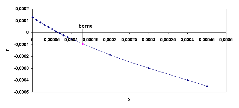
Figure 4-1: Shape of the scalar function
4.3. Coherent tangent operator#
We are trying to calculate: \(\frac{\partial \sigma }{\partial \varepsilon }=\frac{\partial s}{\partial \varepsilon }+\frac{1}{3}\mathrm{Id}\otimes \frac{\partial {I}_{1}}{\partial \varepsilon }\)
With:
\(\frac{\partial s}{\partial \varepsilon }=\frac{\partial {s}^{\mathrm{el}}}{\partial \varepsilon }(1-\frac{3\mu }{{\sigma }_{\text{eq}}^{\mathrm{el}}}\text{.}\Delta p)+\frac{3\mu }{{({\sigma }_{\text{eq}}^{\mathrm{el}})}^{2}}\text{.}\Delta p({s}^{\mathrm{el}}\otimes \frac{\partial {\sigma }_{\text{eq}}^{\mathrm{el}}}{\partial \varepsilon })-\frac{3\mu }{{\sigma }_{\text{eq}}^{\mathrm{el}}}\text{.}({s}^{\mathrm{el}}\otimes \frac{\partial \Delta p}{\partial \varepsilon })\)
\(\frac{\partial {I}_{1}}{\partial \varepsilon }=\frac{\partial {I}_{1}^{\mathrm{el}}}{\partial \varepsilon }-9K\beta (p)\frac{\partial \Delta p}{\partial \varepsilon }\)
Calculation of \(\frac{\partial {s}^{\mathrm{el}}}{\partial \varepsilon }\):
\(\frac{\partial {s}^{\mathrm{el}}}{\partial \varepsilon }=2\mu ({\mathrm{Id}}_{4}-\frac{1}{3}\mathrm{Id}\otimes \mathrm{Id})\)
\(\frac{\mathrm{\partial }{s}_{\text{ij}}}{\mathrm{\partial }{\varepsilon }_{\text{pq}}}\mathrm{=}2\mu ({\delta }_{\text{ip}}{\delta }_{\text{jq}}\mathrm{-}\frac{1}{3}{\delta }_{\text{ij}}{\delta }_{\text{pq}})\)
Calculation of \(\frac{\partial {I}_{1}^{\mathrm{el}}}{\partial \varepsilon }\):
\(\frac{\partial {I}_{1}^{\mathrm{el}}}{\partial \varepsilon }=3K\mathrm{Id}\) is:
\(\frac{\partial {I}_{1}^{\mathrm{el}}}{\partial {\varepsilon }_{\text{pq}}}=3K{\delta }_{\text{pq}}\)
Calculation of \(\frac{\partial {\sigma }_{\text{eq}}^{\mathrm{el}}}{\partial \varepsilon }\):
\(\frac{\partial {\sigma }_{\text{eq}}^{\mathrm{el}}}{\partial \varepsilon }=\frac{\partial {\sigma }_{\text{eq}}^{\mathrm{el}}}{\partial {\sigma }^{\mathrm{el}}}\frac{\partial {\sigma }^{\mathrm{el}}}{\partial \varepsilon }=\frac{\partial {\sigma }_{\text{eq}}^{\mathrm{el}}}{\partial {s}^{\mathrm{el}}}\frac{\partial {s}^{\mathrm{el}}}{\partial {\sigma }^{\mathrm{el}}}\frac{\partial {\sigma }^{\mathrm{el}}}{\partial \varepsilon }=\frac{3}{2}\frac{{s}^{\mathrm{el}}}{{\sigma }_{\text{eq}}^{\mathrm{el}}}({\mathrm{Id}}_{4}-\frac{1}{3}\mathrm{Id}\otimes \mathrm{Id}){D}^{e}=\frac{3}{2}\frac{{s}^{\mathrm{el}}}{{\sigma }_{\text{eq}}^{\mathrm{el}}}{D}^{e}\)
Calculation of \(\frac{\partial \Delta p}{\partial \varepsilon }\):
\(\frac{\Delta p}{\Delta t}=A{\langle \frac{f(\sigma ,p)}{{P}_{\text{ref}}}\rangle }^{n}\)
Be \(F(\Delta p)=\frac{A\Delta t}{{P}_{\mathrm{ref}}^{n}}{\langle f(\sigma ,p)\rangle }^{n}-\Delta p\)
\(\frac{\partial \Delta p}{\partial \varepsilon }=\frac{\partial \Delta p}{\partial {\sigma }^{\mathrm{el}}}\frac{\partial {\sigma }^{\mathrm{el}}}{\partial \varepsilon }\)
To calculate \(\frac{\partial \Delta p}{\partial {\sigma }^{\mathrm{el}}}\), we use \(F({\sigma }^{\mathrm{el}},p)=0\)
\(\frac{\partial F({\sigma }^{\mathrm{el}},p)}{\partial {\sigma }^{\mathrm{el}}}\delta {\sigma }^{\mathrm{el}}+\frac{\partial F({\sigma }^{\mathrm{el}},p)}{\partial \Delta p}\delta \Delta p=0\) from where:
\(\frac{\delta \Delta p}{\delta {\sigma }^{\mathrm{el}}}=-\frac{\frac{\partial F({\sigma }^{\mathrm{el}},p)}{\partial {\sigma }^{\mathrm{el}}}}{\frac{\partial F({\sigma }^{\mathrm{el}},p)}{\partial \Delta p}}\)
\(F(\Delta p)=C{\langle \begin{array}{c}({\sigma }_{\mathrm{eq}}^{\mathrm{el}}+\alpha {I}_{1}^{\mathrm{el}}-{R}^{-})-(3\mu +{R}_{\mathrm{const}}-{\alpha }_{\mathrm{const}}{I}_{1}^{\mathrm{el}}+9K{\alpha }^{-}{\beta }^{-})\Delta p\\ \\ (9K{\alpha }^{-}{\beta }_{\mathrm{const}}+9K{\alpha }_{\mathrm{const}}{\beta }^{-})\Delta {p}^{2}-(9K{\alpha }_{\mathrm{const}}{\beta }_{\mathrm{const}})\Delta {p}^{3}\end{array}\rangle }^{n}-\Delta p=0\)
\(\frac{\partial F({\sigma }^{\mathrm{el}},p)}{\partial {\sigma }^{\mathrm{el}}}=\mathrm{C.}n\mathrm{.}{\langle f({\sigma }^{\mathrm{el}},p)\rangle }^{n-1}\frac{\partial f({\sigma }^{\mathrm{el}},p)}{\partial {\sigma }^{\mathrm{el}}}\)
Where \(\frac{\partial f({\sigma }^{\mathrm{el}},p)}{\partial {\sigma }^{\mathrm{el}}}=(\frac{\partial {\sigma }_{\text{eq}}^{\mathrm{el}}}{\partial {\sigma }^{\mathrm{el}}}+\alpha \frac{\partial {I}_{1}^{\mathrm{el}}}{\partial {\sigma }^{\mathrm{el}}})+{\alpha }_{\text{const}}(\frac{\partial {I}_{1}^{\mathrm{el}}}{\partial {\sigma }^{e}})\Delta p\)
\(\frac{\partial F({\sigma }^{\mathrm{el}},p)}{\partial \Delta p}=\mathrm{C.}n\mathrm{.}{\langle f({\sigma }^{\mathrm{el}},p)\rangle }^{n-1}\frac{\partial f({\sigma }^{\mathrm{el}},p)}{\partial \Delta p}-1\)
\(\begin{array}{}\frac{\partial f({\sigma }^{\mathrm{el}},p)}{\partial \Delta p}=-(3\mu +{R}_{\mathrm{const}}-{\alpha }_{\mathrm{const}}{I}_{1}^{\mathrm{el}}+9K{\alpha }^{-}{\beta }^{-})\\ -2\Delta p9K({\alpha }^{-}{\beta }_{\mathrm{const}}+{\alpha }_{\mathrm{const}}{\beta }^{-})-3\Delta {p}^{2}9K({\alpha }_{\mathrm{const}}{\beta }_{\mathrm{const}})\end{array}\)
Calculation of \(\frac{\partial {\sigma }_{\text{eq}}^{\mathrm{el}}}{\partial {\sigma }^{\mathrm{el}}}\):
\(\frac{\partial {\sigma }_{\text{eq}}^{\mathrm{el}}}{\partial {\sigma }^{\mathrm{el}}}=\frac{\partial {\sigma }_{\text{eq}}^{\mathrm{el}}}{\partial {s}^{\mathrm{el}}}\frac{\partial {s}^{\mathrm{el}}}{\partial {\sigma }^{\mathrm{el}}}=\frac{3}{2}\frac{{s}^{\mathrm{el}}}{{\sigma }_{\text{eq}}^{\mathrm{el}}}\text{.}({I}_{4}-\frac{1}{3}\mathrm{Id}\otimes \mathrm{Id})=\frac{3}{2}\frac{{s}^{\mathrm{el}}}{{\sigma }_{\text{eq}}^{\mathrm{el}}}\)
Calculation of \(\frac{\partial {I}_{1}^{\mathrm{el}}}{\partial {\sigma }^{\mathrm{el}}}\):
\(\frac{\partial {I}_{1}^{\mathrm{el}}}{\partial {\sigma }^{\mathrm{el}}}=\frac{\partial \text{tr}({\sigma }^{\mathrm{el}})}{\partial {\sigma }^{\mathrm{el}}}=\mathrm{Id}\)
4.4. Material data#
The 16 parameters of the model are:
Under ELAS
\(E\): Young’s modulus (\(\mathit{Pa}\) or \(\mathit{MPa}\))
\(\nu\): Poisson’s ratio
Under VISC_DRUC_PRAG
\({P}_{\text{ref}}\): reference pressure (\(\mathit{Pa}\) or \(\mathit{MPa}\))
\(A\): viscoplastic parameter (in \({s}^{\mathrm{-}1}\))
\(n\): power of the creep law
\({p}_{\text{pic}}\): work-hardening rate at the peak threshold
\({p}_{\text{ult}}\): work hardening rate at the ultimate threshold
\({\alpha }_{0}\), \({\alpha }_{\text{pic}}\) and \({\alpha }_{\text{ult}}\): parameters of the cohesion function \(\alpha (p)\)
\({R}_{0}\), \({R}_{\text{pic}}\) and \({R}_{\text{ult}}\): parameters of the work hardening function \(R(p)\)
\({\beta }_{0}\), \({\beta }_{\text{pic}}\) and \({\beta }_{\text{ult}}\): parameters of the dilatance function \(\beta (p)\)
4.5. The internal variables#
\({v}_{1}\mathrm{=}p\): cumulative deviatoric viscoplastic deformation;
\({v}_{2}\mathrm{=}(\text{0 ou 1})\): plasticity indicator;
\({v}_{3}\mathrm{=}\mathit{pos}\): position of the charging point in relation to the threshold:
(\(\text{pos}\mathrm{=}\text{1 si 0}<p<{p}_{\text{pic}}\); \(\text{pos}\mathrm{=}{\text{2 si p}}_{\text{pic}}<p<{p}_{\text{ult}}\); \(\text{pos}\mathrm{=}\text{3 si p}>{p}_{\text{ult}}\))
\({v}_{4}\): number of iterations locally.
4.6. Summary of the resolution algorithm#
The resolution algorithm as implemented in Code_Aster:
\({\sigma }^{\mathrm{el}}={\sigma }^{-}+{D}^{e}\Delta \varepsilon\)
The criterion: \(f({\sigma }^{\mathrm{el}},{p}^{-})={\sigma }_{\text{eq}}^{\mathrm{el}}+\alpha ({p}^{-}){I}_{1}^{\mathrm{el}}-R({p}^{-})\)
Elasticity: if \(f({\sigma }^{\mathrm{el}},{p}^{-})\le 0\) then \(\Delta p\mathrm{=}0\);
Viscoplasticity: if \(f({\sigma }^{\mathrm{el}},{p}^{-})=0\) then \(\Delta p\mathrm{\ge }0\) with \(\Delta p\) solution of equation \(F(\Delta p)\mathrm{=}0\)
where:
\(\frac{\Delta p}{\Delta t}=A{\langle \frac{{\sigma }^{\text{eq}}+\alpha (p){I}_{1}-R(p)}{{P}_{\text{ref}}}\rangle }^{n}=\frac{A}{{P}_{\text{ref}}^{n}}{\langle f(\sigma ,p)\rangle }^{n}\)
and
\(F=\frac{A\Delta t}{{P}_{\mathrm{ref}}^{n}}{\langle f(\sigma ,p)\rangle }^{n}-\Delta p\)
Update the stress tensor:
\(\sigma ={\sigma }^{\mathrm{el}}-{D}^{e}\Delta {\varepsilon }^{\mathrm{vp}}\)
\(s={s}^{\mathrm{el}}(1-3\frac{\mu }{{\sigma }_{\mathrm{eq}}^{\mathrm{el}}}\Delta p)\)
\({\sigma }_{\mathrm{eq}}={\sigma }_{\mathrm{eq}}^{\mathrm{el}}-3G\Delta p\)
\({I}_{1}={{I}_{1}}^{\mathrm{el}}-9K\beta \Delta p\)
\(\sigma =s+\frac{1}{3}{I}_{1}\mathrm{Id}\)
Once \(\Delta p\) is calculated, the constraints and the internal variables updated, we check the position of \(p\) in relation to \({p}^{\mathrm{-}}\) and the sign of \(f(\sigma ,p)\):
If \(0<{p}^{\mathrm{-}}<{p}_{\text{pic}}\); test 1) otherwise 2) otherwise 3)
If \({p}_{\text{pic}}<{p}^{\mathrm{-}}<{p}_{\text{ult}}\); test 2) otherwise 3)
If \({p}^{\mathrm{-}}>{p}_{\text{ult}}\); test 3)
If \({p}^{\mathrm{-}}+\Delta p<{p}_{\text{pic}}\);
we check \(f(\sigma ,p)>0\) with \(R\), \(\mathrm{\alpha }\) and \(\mathrm{\beta }\) corresponding to \(0<p<{p}_{\text{pic}}\),
If \(f(\sigma ,p)>0\) then we update the constraint fields
and internal variables,
otherwise, we consider that \(\Delta p\) is not valid and we re-cut the time step
We check \(f(\sigma ,p)>0\) with \(R\), \(\mathrm{\alpha }\) and \(\beta\) corresponding to \({p}_{\text{pic}}<p<{p}_{\text{ult}}\)
If \(f(\sigma ,p)>0\) then we update the constraint fields
and internal variables,
otherwise, we consider that \(\Delta p\) is not valid and we recut the time step
We check \(f(\sigma ,p)>0\) with \(R\), \(\alpha\) and \(\beta\) corresponding to \(p\mathrm{\ge }{p}_{\text{ult}}\)
If \(f(\sigma ,p)>0\) then we update the constraint fields
and internal variables,
otherwise, we consider that \(\Delta p\) is not valid and we recut the time step