3. Put into equations#

3.1. Formulation of Granger creep in Code_Aster (Reminder)#

In this paragraph, we briefly present the modeling of creep in*Code_Aster*, following the Granger model. For more details, refer to [R7.01.01 et V6.04.142].

The expression of creep deformation applied to a linear viscoelastic material, by applying the Boltzmann Superposition Principle for a non-constant loading history \(\sigma (t)\), can be written in 1D:

\({\epsilon }_{\text{fl}}(t)=\underset{\tau =0}{\overset{t}{\int }}f(t-\tau )\frac{\partial \sigma }{\partial \tau }\mathrm{d\tau }=f\ast \frac{\partial \sigma }{\partial t}\)

\(\ast\) represents the convolution product

\(J(t,{t}_{c})=f(t-{t}_{c})\) is the creep function, an increasing function of \((t-{t}_{c})\) and zero for negative \((t-{t}_{c})\). It can be shown that any linear viscoelastic body can be modelled by a series grouping of Kelvin models and that the creep function can then be put in the form:

\(f(t)=\sum _{s=1}^{r}{J}_{s}(1-\text{exp}(-\frac{t}{{\tau }_{s}}))\)

\({\tau }_{s}\) and \({J}_{s}\) are positive coefficients and identified on the experimental creep curves.

A serial grouping of Kelvin models whose coefficients are identified from experimental creep curves is used. It is shown in practice that concrete creep curves are reproduced with satisfaction with a series of 8 models.

We therefore use the following creep function: \(J(t,{t}_{c})=\sum _{s=1}^{s=8}{J}_{s}(1-\text{exp}(-\frac{t-{t}_{c}}{{\tau }_{s}}))\)

which leads to the expression:

\({\varepsilon }_{\text{fl}}(t)=\underset{\tau =0}{\overset{t}{\int }}\left[\sum _{s=1}^{s=8}{J}_{s}(1-\text{exp}(-\frac{t-\tau }{{\tau }_{s}}))\right]\frac{\partial \sigma }{\partial \tau }d\tau\)

By deriving this expression in the case of a single Kelvin model (s=1), we easily obtain the following equation: \({\tau }_{s}{\dot{\varepsilon }}_{\text{fl}}(t)+{\varepsilon }_{\text{fl}}(t)={J}_{s}\sigma (t)\)

which can also be written as: \(\sigma (t)=\frac{{\tau }_{s}}{{J}_{s}}{\dot{\varepsilon }}_{\text{fl}}(t)+\frac{1}{{J}_{s}}{\varepsilon }_{\text{fl}}(t)\)

or again: \(\sigma (t)=\mu {\dot{\varepsilon }}_{\text{fl}}(t)+K{\varepsilon }_{\text{fl}}(t)\) with \(\mu =\frac{{\tau }_{s}}{{J}_{s}}\) and \(K=\frac{1}{{J}_{s}}\)

We can extend this formulation to the case of the serial development of 8 Kelvin models (or more), with some mathematical developments, which gives:

\(\sigma (t)=\sum _{s=1}^{s=8}\left[{K}_{s}{\varepsilon }_{\text{fl}}^{s}(t)+{m}_{s}{\dot{\varepsilon }}_{\text{fl}}^{s}(t)\right]\)

The rheological model of creep is represented in the figure below, in the case of a single Kelvin model:

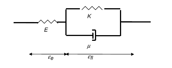
To simplify the presentation of coupling in the following paragraph, we only take into account the first term of the Kelvin serial decomposition, and we write: \(\sigma (t)=\mu {\dot{\varepsilon }}_{\text{fl}}(t)+K{\varepsilon }_{\text{fl}}(t)\)

In addition, for the presentation, we assume \(\mu\) and \(K\) to be constant, i.e. \(\mu ={\mu }^{-}\) and \(K={K}^{-}\) .

3.2. Formulation of the 1D creep/plasticity coupling#

The creep/plasticity coupling corresponds to the rheological model below, where creep, characterized by the coefficients \(K\) and \(\mu\) (stiffness and viscosity), and plasticity are modelled in series.

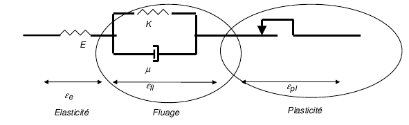
The equations governing creep are as follows:

\(\sigma \mathrm{=}\mu {\dot{\varepsilon }}_{\text{fl}}+K{\varepsilon }_{\text{fl}}\)

\(\varepsilon \mathrm{=}{\varepsilon }_{e}+{\varepsilon }_{\text{fl}}\)

\(\sigma \mathrm{=}E{e}_{\varepsilon }\)

that can be written at the current moment (the exponent “-“designating the previous instant):

\(\varepsilon \mathrm{=}{\varepsilon }_{e}+{\varepsilon }_{\text{fl}}\mathrm{=}{\varepsilon }^{\mathrm{-}}+\Delta {\varepsilon }_{e}+\Delta {\varepsilon }_{\text{fl}}\)

\(\sigma \mathrm{=}\mu {\dot{\varepsilon }}_{\text{fl}}+K{\varepsilon }_{\text{fl}}\mathrm{=}\mu {\dot{\varepsilon }}_{\text{fl}}+K\left[\varepsilon \mathrm{-}{\varepsilon }_{e}\right]\)

\(\sigma \mathrm{=}E{\varepsilon }_{e}\)

The equation governing the plasticity model is as follows:

\(\sigma \mathrm{=}E\left[\varepsilon \mathrm{-}{\varepsilon }_{\text{pl}}\right]\)

This leads, in the case of creep/plasticity coupling, to the following system of equations:

\(\varepsilon \mathrm{=}{\varepsilon }_{e}+{\varepsilon }_{\text{fl}}+{\varepsilon }_{\text{pl}}\mathrm{=}{\varepsilon }^{\mathrm{-}}+\Delta {\varepsilon }_{e}+\Delta {\varepsilon }_{\text{fl}}+\Delta {\varepsilon }_{\text{pl}}\)

\(\sigma \mathrm{=}\mu {\dot{\varepsilon }}_{\text{fl}}+K{\varepsilon }_{\text{fl}}\mathrm{=}\mu {\dot{\varepsilon }}_{\text{fl}}+K\left[\varepsilon \mathrm{-}{\varepsilon }_{e}\mathrm{-}{\varepsilon }_{\text{pl}}\right]\)

\(\sigma \mathrm{=}E{\varepsilon }_{e}\)

\(\sigma \mathrm{=}E\left[\varepsilon \mathrm{-}{\varepsilon }_{\text{pl}}\mathrm{-}{\varepsilon }_{\text{fl}}\right]\)

In the resolution of the behavior equations at the Gauss point, in the elementary routines of Code_Aster, the equality of the constraints resulting from creep and plasticity is not formally written, which in fact corresponds to the following system of equations (noting \({\sigma }_{1}\) the stress resulting from the resolution of creep and \({\sigma }_{2}\) the constraint resulting from the resolution of plasticity at the current moment):

\({\sigma }_{1}\mathrm{=}\mu {\dot{\varepsilon }}_{\text{fl}}+K{\varepsilon }_{\text{fl}}\mathrm{=}\mu {\dot{\varepsilon }}_{\text{fl}}+K\left[\varepsilon \mathrm{-}{\varepsilon }_{e}\mathrm{-}{\varepsilon }_{\text{pl}}\right]\)

\({\sigma }_{1}\mathrm{=}E{\varepsilon }_{e}\)

\({\sigma }_{2}\mathrm{=}E\left[\varepsilon \mathrm{-}{\varepsilon }_{\text{pl}}\mathrm{-}{\varepsilon }_{\text{fl}}\right]\)

However, at the equilibrium of the creep/plasticity coupling, we do indeed have equality between the creep deformation and the plastic deformation in the equations of the Granger creep model, and in the equations of plasticity, which implies, by modifying the equation governing plasticity, we have:

\({\varepsilon }_{e}\mathrm{=}\varepsilon \mathrm{-}{\varepsilon }_{\text{pl}}\mathrm{-}{\varepsilon }_{\text{fl}}\)

then \({\sigma }_{2}\mathrm{=}E\left[\varepsilon \mathrm{-}{\varepsilon }_{\text{pl}}\mathrm{-}{\varepsilon }_{\text{fl}}\right]\mathrm{=}E{\varepsilon }_{e}\)

Hence \({\sigma }_{2}\mathrm{=}E{\varepsilon }_{e}\mathrm{=}{\sigma }_{1}\)

or the equality of the constraints calculated during the resolution of the creep, with the constraints calculated during the resolution of the plasticity: \({\sigma }_{2}={\sigma }_{1}\)

It is the partition of the deformations in the form \(\varepsilon \mathrm{=}{\varepsilon }_{e}+{\varepsilon }_{\text{pl}}+{\varepsilon }_{\text{fl}}\), and the identity of the Young modules of the creep and plasticity models that are at the origin of this result. In fact, the same Young’s modulus intervenes in the creep model and in the plasticity model, and leads, with the identity of the elastic deformation, to the equality of the stresses.

Notes: More generally, this kind of algorithm requires that both laws calculate the elastic stress identical.

Under this hypothesis, a generalization of this coupling to models whose viscous and plastic deformations are additive is possible [1]. We will then write:

\((\begin{array}{c}{\sigma }_{1}\\ {\varepsilon }_{\text{fl}}\end{array})\mathrm{=}{F}_{1}(\varepsilon \mathrm{-}{\varepsilon }_{\text{pl}};{\sigma }^{\mathrm{-}};{\varepsilon }_{\text{pl}}^{\mathrm{-}},\text{.}\text{.}\text{.})\)

\((\begin{array}{c}{\sigma }_{2}\\ {\varepsilon }_{\text{pl}}\end{array})\mathrm{=}{F}_{2}(\varepsilon \mathrm{-}{\varepsilon }_{\text{fl}};{\sigma }^{\mathrm{-}};{\varepsilon }_{\text{fl}}^{\mathrm{-}},\text{.}\text{.}\text{.})\)

A theoretical study of the convergence of such a model, under the assumption that the two behaviors fall within the framework of generalized standard environments, is described in the appendix.

Other coupling possibilities exist, in particular concerning the laws of damage and plasticity [7]. In particular the coupling BETON_UMLV_FP/ENDO_ISOT_BETON is described in [R7.01.06].