7. ANNEXE: convergence of the coupling method#
7.1. Ratings and hypotheses#
In this paragraph and the next, we will consider two nonlinear, dissipative laws of behavior \(\mathrm{L1}\) and \(\mathrm{L2}\) associated with the same elasticity tensor \(H\). The integration of law \(\mathrm{Li}\) consists, at each Gauss point, on the one hand in calculating the stress increment \(\mathrm{Ds}\) and the anelastic deformation increment \(\Delta {\varepsilon }_{{a}_{i}}\) as a function of a total deformation increment \(\Delta \varepsilon\) and of quantities at the beginning of the time step (known) and on the other hand in calculating at point \(\Delta \varepsilon\) the contribution to the tangent operator \({(\frac{\partial \Delta \sigma }{\partial \Delta \varepsilon })}_{\Delta \varepsilon }^{{L}_{i}}\).
We can summarize the « local incremental problem » that is the integration of law \({L}_{i}\) by introducing the \({f}_{i}\) operator defined by:
\((\begin{array}{c}\Delta \sigma \\ \Delta {\varepsilon }_{{a}_{i}}\end{array})={f}_{i}(\Delta \varepsilon )\)
We can then define the \(L\) law of behavior resulting from the coupling of \(\mathrm{L1}\) and \(\mathrm{L2}\). Its anelastic deformation \({\epsilon }_{a}\) is equal to: \({\varepsilon }_{a}={\varepsilon }_{{a}_{1}}+{\varepsilon }_{{a}_{2}}\) and the elasticity relationship associated with \(L\) is written as:
\(\sigma =H(\varepsilon -{\varepsilon }_{{a}_{1}}-{\varepsilon }_{{a}_{2}})\)
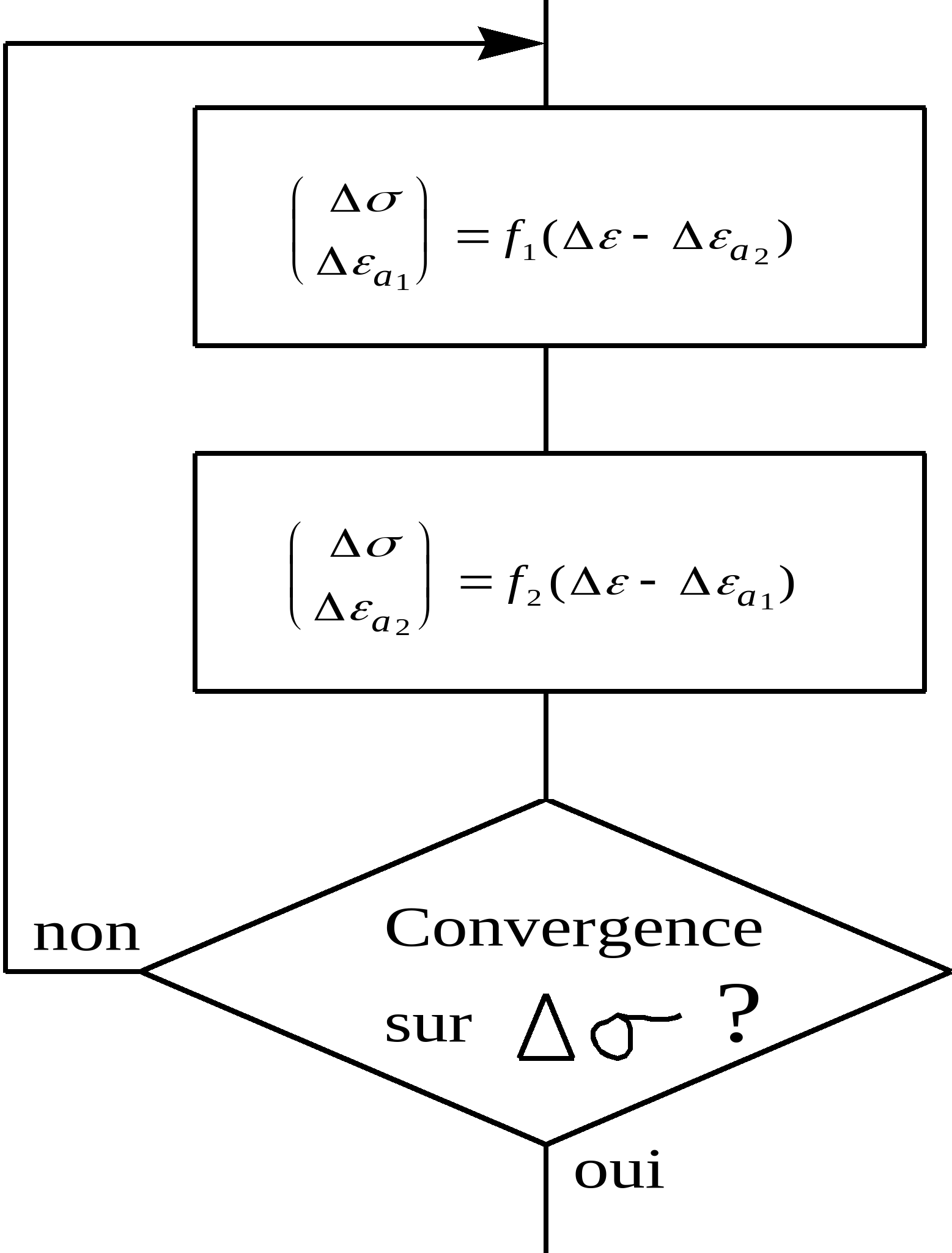
The integration of the law \(L\) is carried out by the successive resolutions of the following « local incremental problems » (laws \({L}_{1}\) and \({L}_{2}\)) in a loop until convergence on \(\Delta \sigma\) (the tangent operator \({(\frac{\partial \Delta \sigma }{\partial \Delta \varepsilon })}_{\Delta \varepsilon }^{L}\) for the law \(L\) is calculated in paragraph 3):
The theoretical approach to this type of coupling has two components:
The convergence study of the loop above
The study of the possibility of putting the global incremental problem (which is structural calculation with law \(L\)) in the form of a minimization problem with a unique solution.
7.2. Writing the global incremental problem in the form of a minimization#
We assume that the two laws of behavior \({L}_{1}\) and \({L}_{2}\) fall within the framework of generalized standard environments. In this case, the « local incremental problem » that is the integration of the \({L}_{i}\) law, described by equality:
\((\begin{array}{c}\Delta \sigma \\ \Delta {\varepsilon }_{{a}_{i}}\end{array})={f}_{i}(\Delta \varepsilon -\Delta {\varepsilon }_{{a}_{j}})\begin{array}{ccc}& & \end{array}\begin{array}{ccc}& & \end{array}({E}_{i})\)
where \(i\in \left\{\mathrm{1,2}\right\}\) and \(j=3-i\), can also be written in the form:
\(\Delta {\varepsilon }_{{a}_{i}}=\text{Arg}\underset{{e}_{i}}{\text{Min}}\left[\phi (\varepsilon +\Delta \varepsilon -\Delta {\varepsilon }_{{a}_{j}},{\varepsilon }_{{a}_{i}}+{\varepsilon }_{{a}_{j}}+{e}_{i})+{G}_{i}({e}_{i})\right]({P}_{i})\)
where \(\varphi\) is the elastic deformation energy:
\(\varphi (\varepsilon ,{\varepsilon }_{a})=\frac{1}{2}H(\varepsilon -{\varepsilon }_{a}):(\varepsilon -{\varepsilon }_{a})\)
and where \({G}_{i}\) is the « complementary potential » of the \({L}_{i}\) law. Below we define this potential \({G}_{i}\) starting from \({f}_{i}\), the stored portion of free energy and a function of the internal variables \({a}_{i}\), and of the dissipation potential \({D}_{i}\), a function of the anelastic deformation rate \({\dot{\varepsilon }}_{{a}_{i}}\) and the rates of evolution of the internal variables \({\dot{\alpha }}_{i}\). With an incremental formulation, we have:
\({G}_{i}({e}_{i})=\underset{\Delta \alpha }{\text{Min}}\left[{\varphi }_{i}({\alpha }_{i}+\Delta \alpha )+{D}_{i}({e}_{i},\Delta \alpha )\right]\)
The vector \({a}_{i}\) of the internal variables of the \({L}_{i}\) law at the start of the time step therefore intervenes as a parameter in the expression for \({G}_{i}\). For each value of this \({a}_{i}\) parameter, the \({G}_{i}\) function is positive and convex.
Note: If there are no internal variables, we simply have \({G}_{i}={D}_{i}\)
It is also assumed that one of the two complementary potentials, \({G}_{1}\) or \({G}_{2}\) , is strictly convex and coercive.
Assuming \(\Delta {\varepsilon }_{{a}_{1}}=\stackrel{ˉ}{x}\), \(\Delta {\varepsilon }_{{a}_{2}}=\stackrel{ˉ}{y}\), and \(F(x,y)=\varphi (\varepsilon +\Delta \varepsilon ,{\varepsilon }_{{a}_{1}}+{\varepsilon }_{{a}_{2}}+x+y)\), the system constituted by equations \(({P}_{1})\) and \(({P}_{2})\) is equivalent to:
\(\{\begin{array}{c}\stackrel{ˉ}{x}=\text{Arg}\underset{x}{\text{Min}}\left[F(x,\stackrel{ˉ}{y})+{G}_{1}(x)\right]\\ \stackrel{ˉ}{y}=\text{Arg}\underset{y}{\text{Min}}\left[F(\stackrel{ˉ}{x},y)+{G}_{2}(y)\right]\end{array}\) (S)
\({G}_{1}\) and \({G}_{2}\) being convex and \(F\) being Cakes-differentiable convex, we have according to the property \(\mathrm{P7}\) of [4] (which follows from proposition 2.2 of Chapter II of [2]):
\((S)\mathrm{\iff }(\stackrel{ˉ}{x},\stackrel{ˉ}{y})\mathrm{=}\text{Arg}\underset{(x,y)}{\text{Min}}\left[F(x,y)+{G}_{1}(x)+{G}_{2}(y)\right]\)
Finding an exact solution to the system formed by equations \(({E}_{1})\) and \(({E}_{2})\) is therefore equivalent to finding the minimum of a continuous, coercive and strictly convex function. According to proposal 1.2 in Chapter II of [2], this minimum exists and is unique.
The local resolution of law \(L\) resulting from the coupling of \({L}_{1}\) and \({L}_{2}\) is therefore equivalent to the minimization problem above. Therefore, \(L\) is a generalized standard law of behavior with j as the elastic deformation energy and \(G\) as the complementary potential, where \(G\) is defined by:
\(G({\dot{\varepsilon }}_{a})={G}_{1}({\dot{\varepsilon }}_{{a}_{1}})+{G}_{2}({\dot{\varepsilon }}_{{a}_{2}})\)
with \({\varepsilon }_{a}={\varepsilon }_{{a}_{1}}+{\varepsilon }_{{a}_{2}}\).
By proceeding in the same way as in §3 of [5], we can therefore put the global incremental problem (which is the calculation of structure with the \(L\) law) in the form of a minimization problem with a unique solution.
7.3. Algorithm convergence#
It is now necessary to prove that the algorithm described above converges well.
We write \({z}_{n}=({x}_{n},{y}_{n})=(\Delta {\varepsilon }_{a}^{{n}_{1}},\Delta {\varepsilon }_{a}^{{n}_{2}})\) the result from iteration \(n\) and we ask:
\(K(z)\mathrm{=}K(x,y)\mathrm{=}F(x,y)+{G}_{1}(x)+{G}_{2}(y)\)
We calculate \({z}_{n+1}\) as a function of \({z}_{n}\) in the following way:
\(\begin{array}{}{x}_{n+1}=\text{Arg}\underset{x}{\text{Min}}K(x,{y}_{n})\\ {y}_{n+1}=\text{Arg}\underset{y}{\text{Min}}K({x}_{n+1},y)\end{array}\)
We note:
\(\stackrel{ˉ}{z}=(\stackrel{ˉ}{x},\stackrel{ˉ}{y})=\text{Arg}\underset{(x,y)}{\text{Min}}K(x,y)\)
To show the convergence of the sequence \(({z}_{n})\) to \(\stackrel{ˉ}{z}\), we will use the global convergence theorem from §6.5 of [3].
We consider \(A\) to be the algorithm that, starting with a given \({z}_{0}\), generates the sequence \(({z}_{n})\) defined above:
\({z}_{n+1}=A({z}_{n})\)
The solution set \(\Gamma\) consists of the singleton {\(\stackrel{ˉ}{z}\)}.
Let’s check the hypotheses of this theorem:
H1: all points \({z}_{n}\) are contained in a compact set \(S\) .
By construction, we have:
\(\mathrm{\forall }n\mathrm{\in }\mathrm{\mathbb{N}},K({z}_{n})\mathrm{\le }K({z}_{0})\)
Now, \(K\) is coercive so \(K(z)\underset{\mathrm{\parallel }z\mathrm{\parallel }\to +\mathrm{\infty }}{\to }+\mathrm{\infty }\) with \({\mathrm{\parallel }z\mathrm{\parallel }}^{2}\mathrm{=}{x}_{\text{eq}}^{2}+{y}_{\text{eq}}^{2})\)
So:
\(\mathrm{\forall }R>0\), \(\mathrm{\exists }M>0\), \(\mathrm{\forall }z\), \(\mathrm{\parallel }z\mathrm{\parallel }>M\mathrm{\Rightarrow }K(z)>R\)
\(\mathrm{\forall }R>0\), \(\mathrm{\exists }M>0\), \(\mathrm{\forall }z\), \(K(z)\mathrm{\le }R\mathrm{\Rightarrow }\mathrm{\parallel }z\mathrm{\parallel }\mathrm{\le }M\)
By taking \(R\mathrm{=}K({z}_{0})\), we therefore have:
\(\forall n\in \mathbb{N},∣∣{z}_{n}∣∣\le M\)
So all points \({z}_{n}\) are contained in a bounded set, therefore in a compact since the vector space is finite in dimension, so the hypothesis is satisfied.
H2. There is a descent function \(Z\) for \(\Gamma\) and \(A\)
\(Z\) should be continuous and check for the following two properties:
. if \(z\mathrm{\ne }\stackrel{ˉ}{z}\), then \(Z(A(z))<Z(z)\)
. if \(z\mathrm{=}\stackrel{ˉ}{z}\), then \(Z(A(z))\mathrm{\le }Z(z)\)
We take \(Z\mathrm{=}K\)
\(K\) is well ongoing and we have:
. \(K(A(\stackrel{ˉ}{z}))\mathrm{=}K(\stackrel{ˉ}{z})\)
. If \(z\mathrm{\ne }\stackrel{ˉ}{z}\), then \(A(z)\mathrm{=}z’\mathrm{=}(x’,y’)\) such as:
\(\begin{array}{c}x\text{'}\mathrm{=}\text{Arg}\underset{x}{\text{Min}}K(x,y)\\ y\text{'}\mathrm{=}\text{Arg}\underset{y}{\text{Min}}K(x\text{',}y)\end{array}\)
If we have \(x’\mathrm{\ne }x\), then \(K\) being continuous, coercive and strictly convex, the minimum \(x’\) is unique and we have
\(K(x’,y)<K(x,y)\). Now, we have \(K(x’,y’)\mathrm{\le }K(x’,y)\) so \(K(z’)<K(z)\).
If we have \(x’\mathrm{=}x\), then we have \(y’\mathrm{\ne }y\) (if not, we would have \(z\mathrm{=}\stackrel{ˉ}{z}\)).
\(K\) being continuous, coercive and strictly convex, the minimum \(y’\) is unique and we have:
\(K(x’,y’)<K(x’,y)\mathit{et}K(x’,y)\mathrm{=}K(x,y)\) so \(K(x’,y’)<K(x,y)\)
So in both cases we have:
\(K(A(z))<K(z)\)
So there is a descent function for \(\Gamma\) and \(A\). The hypothesis is satisfied.
H3. The algorithm \(A\) is closed for everything \(z\) that does not belong to \(\Gamma\)
To verify this third hypothesis, we will adopt the same method as that used in §7.8 of [3] to show the global convergence of a cyclic coordinate descent algorithm.
Consider the following two algorithms:
\({C}^{1}\) which at \((x,y)\) associates all the points \((X,y)\) with any \(X\)
\({C}^{2}\) which at \((x,y)\) associates all the points \((x,Y)\) with any \(Y\)
In addition, we consider \(M\) the minimization algorithm on each of these two sets (which associates the point achieving the minimum on the set with one element of the set). Algorithm \(A\) is then the composition of 4 algorithms:
\(A\mathrm{=}M{C}^{2}M{C}^{1}\)
Algorithms \({C}^{1}\) and \({C}^{2}\) are continuous and \(M\) is closed. As all the points are contained in a compact set \(S\) (cf the first hypothesis), we deduce from corollary 1 of §6.5 of [3] that \(A\) is closed, so the hypothesis is satisfied.
The three hypotheses of the global convergence theorem having been verified, we have therefore shown the following result:
The limit of any convergent subsequence of \(({z}_{n})\) is \(\stackrel{ˉ}{z}\) . \((P)\)
However, we have also shown that all the \({z}_{n}\) points are contained in a \(S\) compact. Assume that \(({z}_{n})\) does not converge to \(\stackrel{ˉ}{z}\), then we have:
\(\mathrm{\exists }\varepsilon >\mathrm{0,}\mathrm{\forall }N\mathrm{\in }\mathrm{\mathbb{N}},\mathrm{\exists }n\mathrm{=}\psi (N)>N,\mathrm{\parallel }{z}_{n}\mathrm{-}\stackrel{ˉ}{z}\mathrm{\parallel }>\varepsilon\)
We can build a sub-suite \(({z}_{b(n)})\) defined by:
\(b(0)\mathrm{=}0\)
\(\mathrm{\forall }n\mathrm{\in }\mathrm{\mathbb{N}},\beta (n+1)\mathrm{=}\psi (\beta (n))\)
So we have: \(\mathrm{\forall }n\mathrm{\in }\mathrm{\mathbb{N}},∣∣{z}_{\beta (n)}\mathrm{-}\stackrel{ˉ}{z}∣∣\mathrm{\le }M\)
However, the set \((S–B(\stackrel{ˉ}{z},e))\) is compact, so the sequence \(({z}_{b(n)})\) has a convergent subsequence which, according to the property \((P)\) above, converges to \(\stackrel{ˉ}{z}\), which is absurd.
The desired result is therefore obtained:
The seque \(({z}_{n})\) converges to \(\stackrel{ˉ}{z}\) .
7.4. Calculation of the tangent operator#
By noting \(\Delta \varepsilon\) the total deformation increment (as an input for the \(L\) law resulting from the coupling of \({L}_{1}\) and \({L}_{2}\)), we can explicitly calculate the tangent operator of \(L\) evaluated at point \(\Delta \varepsilon\), an operator that we note \({(\frac{\mathrm{\partial }\Delta \sigma }{\mathrm{\partial }\Delta \varepsilon })}_{\Delta \varepsilon }^{L}\):
\(\begin{array}{c}{(\frac{\mathrm{\partial }\Delta \sigma }{\mathrm{\partial }\Delta \varepsilon })}_{\Delta \varepsilon }^{L}\mathrm{=}{(\frac{\mathrm{\partial }\Delta \sigma }{\mathrm{\partial }\Delta \varepsilon })}_{\Delta \varepsilon \mathrm{-}\Delta {\varepsilon }_{{a}_{2}}}^{{L}_{1}}\frac{\mathrm{\partial }(\Delta \varepsilon \mathrm{-}\Delta {\varepsilon }_{{a}_{2}})}{\mathrm{\partial }\Delta \varepsilon }\\ {(\frac{\mathrm{\partial }\Delta \sigma }{\mathrm{\partial }\Delta \varepsilon })}_{\Delta \varepsilon }^{L}\mathrm{=}{(\frac{\mathrm{\partial }\Delta \sigma }{\mathrm{\partial }\Delta \varepsilon })}_{\Delta \varepsilon \mathrm{-}\Delta {\varepsilon }_{{a}_{2}}}^{{L}_{1}}({H}^{\mathrm{-}1}{(\frac{\mathrm{\partial }\Delta \sigma }{\mathrm{\partial }\Delta \varepsilon })}_{\Delta \varepsilon }^{L}+\frac{\mathrm{\partial }\Delta {\varepsilon }_{{a}_{1}}}{\mathrm{\partial }\Delta \varepsilon })\begin{array}{ccc}& & \end{array}(3\text{.}1)\end{array}\)
where \(\Delta {\varepsilon }_{{a}_{i}}\) results from the convergence of the loop described in paragraph 7, with \(\Delta \varepsilon\) as input. Now, by symmetry on the indices 1 and 2, we also have:
\(\begin{array}{c}{(\frac{\mathrm{\partial }\Delta \sigma }{\mathrm{\partial }\Delta \varepsilon })}_{\Delta \varepsilon }^{L}\mathrm{=}{(\frac{\mathrm{\partial }\Delta \sigma }{\mathrm{\partial }\Delta \varepsilon })}_{\Delta \varepsilon \mathrm{-}\Delta {\varepsilon }_{{a}_{1}}}^{{L}_{2}}\frac{\mathrm{\partial }(\Delta \varepsilon \mathrm{-}\Delta {\varepsilon }_{{a}_{1}})}{\mathrm{\partial }\Delta \varepsilon }\\ {(\frac{\mathrm{\partial }\Delta \sigma }{\mathrm{\partial }\Delta \varepsilon })}_{\Delta \varepsilon }^{L}\mathrm{=}{(\frac{\mathrm{\partial }\Delta \sigma }{\mathrm{\partial }\Delta \varepsilon })}_{\Delta \varepsilon \mathrm{-}\Delta {\varepsilon }_{{a}_{1}}}^{{L}_{2}}(I\mathrm{-}\frac{\mathrm{\partial }\Delta {\varepsilon }_{{a}_{1}}}{\mathrm{\partial }\Delta \varepsilon })\end{array}\)
So we can calculate \((\frac{\mathrm{\partial }\Delta {\varepsilon }_{{a}_{1}}}{\mathrm{\partial }\Delta \varepsilon })\): \(\frac{\mathrm{\partial }\Delta {\varepsilon }_{{a}_{1}}}{\mathrm{\partial }\Delta \varepsilon }\mathrm{=}I\mathrm{-}{\left[{(\frac{\mathrm{\partial }\Delta \sigma }{\mathrm{\partial }\Delta \varepsilon })}_{\Delta \varepsilon \mathrm{-}\Delta {\varepsilon }_{{a}_{1}}}^{{L}_{2}}\right]}^{\mathrm{-}1}{(\frac{\mathrm{\partial }\Delta \sigma }{\mathrm{\partial }\Delta \varepsilon })}_{\Delta \varepsilon }^{L}\)
By introducing this expression into equation (3.1), we obtain:
\({(\frac{\mathrm{\partial }\Delta \sigma }{\mathrm{\partial }\Delta \varepsilon })}_{\Delta \varepsilon }^{L}\mathrm{=}{(\frac{\mathrm{\partial }\Delta \sigma }{\mathrm{\partial }\Delta \varepsilon })}_{\Delta \varepsilon \mathrm{-}\Delta {\varepsilon }_{{a}_{2}}}^{{L}_{1}}({H}^{\mathrm{-}1}{(\frac{\mathrm{\partial }\Delta \sigma }{\mathrm{\partial }\Delta \varepsilon })}_{\Delta \varepsilon }^{L}+I\mathrm{-}{\left[{(\frac{\mathrm{\partial }\Delta \sigma }{\mathrm{\partial }\Delta \varepsilon })}_{\Delta \varepsilon \mathrm{-}\Delta {\varepsilon }_{{a}_{1}}}^{{L}_{2}}\right]}^{\mathrm{-}1}{(\frac{\mathrm{\partial }\Delta \sigma }{\mathrm{\partial }\Delta \varepsilon })}_{\Delta \varepsilon }^{L})\)
From where:
\(\left[I\mathrm{-}{(\frac{\mathrm{\partial }\Delta \sigma }{\mathrm{\partial }\Delta \varepsilon })}_{\Delta \varepsilon \mathrm{-}\Delta {\varepsilon }_{{a}_{2}}}^{{L}_{1}}({H}^{\mathrm{-}1}\mathrm{-}{\left[{(\frac{\mathrm{\partial }\Delta \sigma }{\mathrm{\partial }\Delta \varepsilon })}_{\Delta \varepsilon \mathrm{-}\Delta {\varepsilon }_{{a}_{1}}}^{{L}_{2}}\right]}^{\mathrm{-}1})\right]{(\frac{\mathrm{\partial }\Delta \sigma }{\mathrm{\partial }\Delta \varepsilon })}_{\Delta \varepsilon }^{L}\mathrm{=}{(\frac{\mathrm{\partial }\Delta \sigma }{\mathrm{\partial }\Delta \varepsilon })}_{\Delta \varepsilon \mathrm{-}\Delta {\varepsilon }_{{a}_{2}}}^{{L}_{1}}\)
So we finally have:
\({(\frac{\mathrm{\partial }\Delta \sigma }{\mathrm{\partial }\Delta \varepsilon })}_{\Delta \varepsilon }^{L}\mathrm{=}{\left[{\left[{(\frac{\mathrm{\partial }\Delta \sigma }{\mathrm{\partial }\Delta \varepsilon })}_{\Delta \varepsilon \mathrm{-}\Delta {\varepsilon }_{{a}_{2}}}^{{L}_{1}}\right]}^{\mathrm{-}1}+{\left[{(\frac{\mathrm{\partial }\Delta \sigma }{\mathrm{\partial }\Delta \varepsilon })}_{\Delta \varepsilon \mathrm{-}\Delta {\varepsilon }_{{a}_{1}}}^{{L}_{2}}\right]}^{\mathrm{-}1}\mathrm{-}{H}^{\mathrm{-}1}\right]}^{\mathrm{-}1}\)