10. Bibliography#
COUSSY: « Mechanics of porous media ». TECHNIP editions.
GERMAIN: « Course in the mechanics of continuous media ».
DUVAUT, J. L. LIONS: « Inequalities in mechanics and physics ».
CHAVANT, P. CHARLES, Th. DUFORESTEL, F. VOLDOIRE: « Thermo-hydro-mechanics of unsaturated porous media in Code_Aster ». Note HI-74/99/011/A.
« Quasi-static nonlinear algorithm (operator STAT_NON_LINE) » Aster Document [R5.03.01]
« Behavior Models THHM » Aster Document [R7.01.11] Index A
GIRAUD: « Adaptation to the nonlinear poroelastic model of Lassabatère-Coussy to modeling unsaturated porous media », (ENSG).
WABINSKI, F. VOLDOIRE: Thermohydromechanics in a saturated medium. Note EDF/DER HI‑74/96/010, from September 1996.
LASSABATERE: « Hydromechanical couplings in an unsaturated porous medium with phase change: application to the desiccation shrinkage of concrete ». Thesis ENPC.
Ph. MESTAT, M. PRAT: « Books in interaction ». Hermes
et al. THILUS: « Poro-mechanics », Biot Conference 1998.
CROUZEIX and MIGNOT, MASSON: « Numerical analysis of differential equations » 1992
« Transient thermal algorithm » Aster Document [R5.02.01].
« Diagonalization of the thermal mass matrix » Aster Document [R3.06.07].
O.C. ZIENKIEWICZ, C.T. CHANG, P. BETTESS: Drained, undrained, consolidating dynamic behaviour assumptions in soils. Geotechnics, 30, pp. 385-395, 1980.
P1P1 one-dimensional problem
We consider a one-dimensional consolidation problem whose unknowns vary only according to the single space variable \(x\).
A rectangular domain of length \(L\) is filled with a porous material with Lamé coefficients \(\lambda\) and \(\mu\), with a Biot coefficient \(b\) and with a Biot module \(N=\frac{1}{M}\) and with hydraulic conductivity \({\lambda }_{h}\). The density of the fluid is noted \(\rho\). We note \(\sigma\) the stress \({\sigma }_{\text{xx}}\), \(u\) the displacement in the direction \(x\), the displacement in the direction, \(\varepsilon =\frac{\partial u}{\partial x}\) the deformation, \(p\) the pressure, \(m\) the mass supply of fluid, \(M\) the flow of fluid.
The boundary conditions are:
in \(x=0\): \(\sigma =0;p=0\)
in \(x=L\): \(u=0;p=1\) for \(t>0\)
The initial conditions in \(t=0\) are \(\mathrm{\sigma }=u=p=0\).

The equation gives:
Mechanical balance and linear elasticity: \(\sigma =(\lambda +2\mu )\varepsilon -\text{bp}=0\)
Mass conservation: \(\frac{\partial m}{\partial t}+\frac{\partial M}{\partial x}=0\)
Darcy’s law: \(M=-{\lambda }_{h}\rho \frac{\partial p}{\partial x}\)
Couplings: \(\frac{m}{\rho }=\text{Np}+b\varepsilon\)
We do an implicit time discretization and we are interested in calculating the first time step:
We get the system of two equations:
\(\{\begin{array}{}\sigma =(\lambda +2\mu )\varepsilon (u)-\text{bp}=0\\ \text{Np}+b\varepsilon -{\lambda }_{h}\Delta t \Delta p =0\end{array}\)
The mixed variational formulation of this problem is:
:math:`{begin{array}{}{int }_{Omega }left[(lambda +2mu )varepsilon (u)varepsilon ({u}^{text{*}})-text{bp}varepsilon ({u}^{text{*}})right]=0forall {u}^{text{*}}\ {int }_{Omega }left[{text{Npp}}^{text{*}}+bvarepsilon (u){p}^{text{*}}+{lambda }_{h}Delta t nabla pnabla {p}^{text{*}}right]=0forall {p}^{text{*}}end{array}`**eq Year 1-1**
Regarding spatial discretization, we cut the medium into \(n\) finite elements. The nodes for element \(i\) are \(i\) and \(i+1\). We note \({u}_{e}^{1}\) and \({p}_{e}^{1}\) the movement and the pressure of the first node of the element \(e\), \({u}_{e}^{2}\) and \({p}_{e}^{2}\) the movement and the pressure of its second node. It is assumed that we use P1P1 finite elements, i.e. that the displacements as well as the pressures are interpolated linearly. Discretizing the first equation then gives:
\(\sum _{e}\frac{{u}_{e}^{\text{*}2}-{u}_{e}^{\text{*}1}}{\Delta x }\left[(\lambda +2\mu )\frac{{u}_{e}^{2}-{u}_{e}^{1}}{\Delta x }-b\frac{{p}_{e}^{1}+{p}_{e}^{2}}{2}\right]=0\)
From which we deduce:
\(({u}_{e}^{2}-{u}_{e}^{1})=\frac{b\Delta x }{\lambda +2\mu }\frac{{p}_{e}^{1}+{p}_{e}^{2}}{2}\text{}\forall e\) eq Year 1-2
Discretizing the second equation gives:
\(\sum _{e}\frac{{p}_{e}^{\text{*}2}+{p}_{e}^{\text{*}1}}{2}\left[b\frac{{u}_{e}^{2}-{u}_{e}^{1}}{\Delta x }+N\frac{{p}_{e}^{1}+{p}_{e}^{2}}{2}\right]+{\lambda }_{h}\Delta t \sum _{e}\frac{{p}_{e}^{\text{*}2}-{p}_{e}^{{\text{*}}^{1}}}{\Delta x }\frac{{p}_{e}^{2}-{p}_{e}^{1}}{\Delta x }=0\)
Putting [éq An 1-2] on it, we find:
\(\sum _{e}\frac{{p}_{e}^{\text{*}2}+{p}_{e}^{\text{*}1}}{2}(N+\frac{{b}^{2}}{\lambda +2\mu })\frac{{p}_{e}^{1}+{p}_{e}^{2}}{2}+{\lambda }_{h}\frac{\Delta t }{\Delta {x}^{2}}\sum _{e}({p}_{e}^{\text{*}2}-{p}_{e}^{\text{*}1})({p}_{e}^{2}-{p}_{e}^{1})=0\) eq Year 1-3
If now, we make the time step tend to zero with no constant space, \({\lambda }_{h}\frac{\Delta t }{\Delta {x}^{2}}\text{<<}(N+\frac{{b}^{2}}{\lambda +2\mu })\), and [éq An 1-3] is reduced to:
\(\sum _{e}({p}_{e}^{\text{*}2}+{p}_{e}^{\text{*}1})({p}_{e}^{1}+{p}_{e}^{2})=0\)
A global numbering of nodes and pressure unknowns is introduced:
\({p}_{j}^{1}={p}_{j};{p}_{j}^{2}={p}_{j+1}\)
We can see that this set of relationships finally gives:
\(\{\begin{array}{}{p}_{1}=0\\ {p}_{i}+2{p}_{i+1}+{p}_{i+2}=0\forall i\in \left[\mathrm{1,}n-1\right]\\ {p}_{n+1}=1\end{array}\)
The solution in this suite is:
\(\{\begin{array}{}{p}_{2j-1}=\frac{j-1}{n}\\ {p}_{2j}=-\frac{2j-1}{2n}\end{array}\)
This gives the following pressure distribution:

As an indication, we give below a comparison of numerical results obtained with elements \(\mathit{P1P1}\), \(\mathit{P2P2}\) and \(\mathit{P2P1}\).
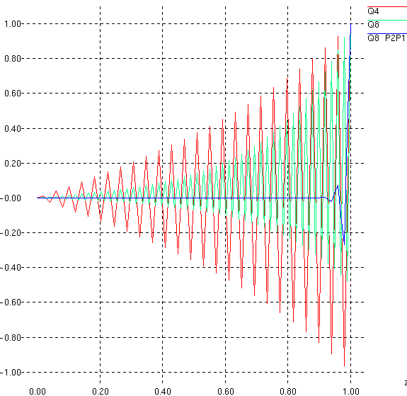
We can see that element \(\mathit{P2P1}\) does not take away the oscillation, but attenuates it appreciably.