4. Procedure for calculating nonlinear modes

We are looking for the periodic solutions of the system

(4.1)\[\begin{split} \ {\ begin {array} {c}\ mathrm {M}\ text {.} \ ddot {\ mathrm {U}} (t) +\ mathrm {K}\ mathrm {K}\ mathrm {K} (t) +\ left (\ begin {array} {c} 0\\ {\ mathrm {F}}}} (t)\ end {array} {F}}} (t)\ end {array}\ right) =\ mathrm {F}}}}} ^ {\ mathrm {F}}}}} ^ {\ mathrm {nl}}} ^ {\ mathrm {nl}}} (\ mathrm {nl}}} (t))\ end {array}\ right) =\ mathrm {F}}}}} ^ {\ mathrm {F}}}}} ^ {\ mathrm {}\\\ mathrm {G} ({\ mathrm {U}}}} ^ {\ mathrm {nl}} (t), {\ mathrm {F}} ^ {\ mathrm {nl}} (t) (t) (t),\ mathrm {U}}}} ^ {\ mathrm {nl}} (t) ^ {\ mathrm {nl}} (t) ^ {\ mathrm {nl}} (t) (t),\ mathrm {nl}} (t) (t),\ mathrm {nl}} (t) =\ mathrm {0,}\ end {nl}} (t) (t)\end{split}\]

by writing the vector \(\mathrm{U}(t)\) using a Fourier series that is truncated to order \({H}_{l}\) (assuming that the influence of higher harmonics is negligible), or

(4.2)\[ \ mathrm {U} (t) = {\ mathrm {U}}} _ {0}} _ {0} +\ sum _ {k=1} ^ {{H} _ {l}} {\ mathrm {U}}} _ {\ mathrm {Ck}} _ {\ mathrm {Ck}}} _ {\ mathrm {Ck}}} _ {\ mathrm {Ck}}}\ mathrm {sin} (k\ omega t)\ mathrm {.}\]

The same expansion is carried out for the unknown vectors \({\mathrm{F}}^{\mathrm{nl}}(t)\) and \(\mathrm{Z}(t)\), but with a different truncation order, which is called \({H}_{\mathit{nl}}\). Then he comes

(4.3)\[\begin{split} \ {\ begin {array} {c} {\ mathrm {fr}}} {\ mathrm {F}}} ^ {\ mathrm {nl}} (t) = {\ mathrm {f}} _ {0} ^ {\ mathrm {nl}} ^ {\ mathrm {nl}}} {\ mathrm {nl}}} {\ mathrm {F}}} +\ sum _ {k=1}} ^ {k=1} ^ {{H}} _ {\ mathrm {F}}} _ {\ mathrm {F}}} _ {\ mathrm {F}}} {Ck}} ^ {\ mathrm {nl}}}\ mathrm {cos} (k\ omega t) + {\ mathrm {F}}} _ {\ mathrm {Sk}} ^ {\ mathrm {nl}}}\ mathrm {nl}}}}\ mathrm {nl}}}}\\ mathrm {nl}}}}\\ mathrm {nl}}}}\\ mathrm {nl}}}}\ mathrm {sin} (k\ omega t),\\ mathrm {Z} (t) = {\ mathrm {Z}}} _ {0} +\ sum _ {k=1} ^ {{H} _ {{H} _ {\ mathit {nl}}}} {\ mathrm {Z}} _ {\ mathrm {Ck}}\ mathrm {cos} (k\ omega t) + {\ mathrm {H}} _ {\ mathrm {z}}} _ {\ mathrm {Sk}}\ mathrm {sin}}\ mathrm {sin} (k\ omega t) (k\ omega t)\ mathrm {.} \ end {array}\end{split}\]

Note Bene: The choice of different order is a direct result of the quantities represented. For a system that is not very shocking, in the vicinity of the linear mode, the answer \(\mathrm{U}(t)\) will be close to a pure sine. A low harmonic number will therefore be chosen. We will increase \({H}_{l}\) when looking for solutions associated with high energy levels. On the other hand, even for low shock forces, the spectral content can be significant, especially if the shock is steep. It will therefore be necessary to remember a large number of harmonics, and we will therefore generally have \({H}_{\mathit{nl}}\gg {H}_{l}\) * . *

In practice, you can start to perform a calculation by choosing relatively low orders, to get an idea of the main behavior. On the other hand, with a low harmonic number, we will not be able to capture the bifurcations correctly. We will therefore gradually increase the values of \({H}_{l}\) and \({H}_{\mathit{nl}}\) to reveal more complex behaviors.

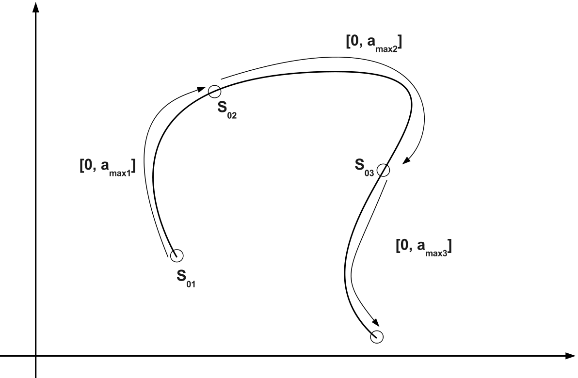
After having performed harmonic balancing, we obtain a sub-determined algebraic system whose unknowns are the Fourier coefficients of \(\mathrm{U}(t)\), \({\mathrm{F}}^{\mathrm{nl}}(t)\) and \(\mathrm{Z}(t)\) and the additional unknown, the natural pulsation \(\omega\). We group these unknowns into a single vector in order to put the system in the form (). We can then use MAN as indicated in the reference [Bib3]. To do this, we expand the unknown vector \(S\) into an integer series according to a path parameter \(a\)

(4.4)\[ S (a) = {S} _ {0} +\ sum _ {k=1} ^ {{N} _ {\ mathit {MAN}}}} {a} ^ {k} {k} {S} {S} _ {k},\]

where \({S}_{0}\) corresponds to the initialization vector of the algorithm, and \({S}_{k}\) for \(k=\mathrm{1,}\dots ,{N}_{\mathit{MAN}}\) are the coefficients of the entire series that remain to be determined. Next, we develop the function \(R\) in a Taylor series, in the vicinity of the initialization vector \({S}_{0}\)

(4.5)\[ 0=R (S (a)) =R ({S} _ {0}) +\ frac {\ mathit {dR}} {\ mathit {dS}} ({S} _ {0})\ left (\ sum _ {k=1}} ^ {k=1}} ^ {k} {0})\ left (\ sum _ {k=1}} ^ {k}\ right) +\ frac {\ mathit {dR}}} {\ mathit {dS}}} ({S} _ {0})\ left (\ sum _ {k=1}}} ^ {k}\ right) +\ frac {\ mathit {dR}}} {\ mathit {dR}}} {\ mathit {dS}} {0}) = R (S ac {{d} ^ {2} R} {{\ mathit {dS}}} ^ {dS}}} ^ {2}} ({S} _ {0})\ left (\ sum _ {k=1} ^ {{N} _ _ {N} _ {1} _ {n} _ {1} _ {1} _ {\ n} _ {1} _ {\ mathit {MAN}}} {a} ^ {l} {l} {s} _ {l}\ right) MAN MAN\]

This relationship is true regardless of \(a\), we then move on to the resolution of a series of \({N}_{\mathit{MAN}}\) linear systems having the same tangent matrix, depending on each other recursively. The resolution of these systems makes it possible to obtain the vectors \({S}_{k}\). Note that we can calculate this matrix analytically because the function \(R\) is quadratic, i.e.

(4.6)\[ \ frac {\ mathit {dR}} {\ mathit {dS}}} ({S} _ {0}) {e} _ {i} =L ({e} _ {i}) +Q ({e} _ {i}, {i}, {i}, {i}, {i}, {i}, {i}, {i}) +Q ({S} _ {0}) +Q ({e} _ {i}) +Q ({e} _ {i}) +Q ({e} _ {i}),\]

where \({e}_{i}\) is the canonical base vector. We thus obtain a branch of solutions \(S(a)\) with \(a\in [\mathrm{0,}{a}_{\mathit{max}}]\), where \({a}_{\mathit{max}}\) represents the domain of validity of the entire series. Therefore, it is possible to obtain the branches of periodic solutions that form the non-linear modes of the model.

The method also makes it possible to locate simple bifurcations by detecting a geometric series in the entire serial representation.