3. Modeling

It is assumed that in the absence of contacts, the structure studied behaves linearly and that the equations governing its dynamic equilibrium have been discretized by finite differences or by finite elements. We obtain a discrete system of second-order differential equations with \(n\) degrees of freedom.

In general, these equations take the following form:

\(\mathrm{M}\text{.}\ddot{\mathrm{U}}(t)+\mathrm{K}\text{.}\mathrm{U}(t)+{\mathrm{F}}^{\mathrm{nl}}(\mathrm{U}(t))=\mathrm{0,}\)

• \(\mathrm{M}\) is the mass matrix of the system,

• \(K\) is the elastic stiffness matrix of the system,

• \({\mathrm{F}}^{\mathrm{nl}}\) is the vector of non-linear shock forces,

We place ourselves in the framework of localized nonlinearities, that is to say that the forces apply to a relatively small number of degrees of freedom. We will note \({I}_{\mathit{nl}}\) the set of indices of these degrees of freedom, and \({I}_{l}\) its complement, that is to say \({I}_{n}=\{\mathrm{1,}\dots ,n\}={I}_{\mathit{nl}}\cup {I}_{l}\). The size of vector \({I}_{\mathit{nl}}\) is equal to \({n}_{\mathit{nl}}\).

To be able to use algorithm EHMAN, which combines the harmonic balancing method (EH) and the numerical asymptotic method (MAN), it is necessary to adopt a certain formalism. This consists in rewriting the problem in the form of a system of order one, with non-linearities at most quadratic, i.e. a system of unknown \(S\) of the form

(3.1)\[ A (\ dot {S}) =C+L (S) +Q (S, S),\]

where \(C\) is a constant, \(L\) is a linear form, and \(Q\) is a quadratic form. The terms on the right-hand side are generally grouped under the name \(R(S)\), so the problem to be solved is then put into a condensed form.

(3.2)\[ A (\ dot {S}) =R (S)\]

To do this, two additional unknown vectors \({\mathrm{F}}^{\mathrm{nl}}(t)\) and \(\mathrm{Z}(t)\) are introduced, as well as additional equations to define these vectors. The vector \({\mathrm{F}}^{\mathrm{nl}}(t)\) describes the contact force and the vector \(\mathrm{Z}(t)\) is called the vector of auxiliary variables. Vector \(\mathrm{Z}(t)\) is \({n}_{z}\) in size. This relatively abstract rewriting, detailed through examples, leads to the solution of a system of the form

(3.3)\[\begin{split} \ {\ begin {array} {c}\ dot {\ mathrm {U}} (t) =\ mathrm {V} (t),\\ mathrm {M}\ text {.} \ dot {\ mathrm {V}} (t) =-\ mathrm {K}\ mathrm {K}\ mathrm {K} (t) -\ left (\ begin {array} {c} 0\\ {\ mathrm {F}}} (t)\ {\ mathrm {F}}} (t)\ {\ mathrm {F}}} (t) ^ {\ mathrm {F}}}}} ^ {\ mathrm {F}}}}} ^ {\ mathrm {nl}}} ^ {\ mathrm {nl}}} (\ mathrm {nl}}} (t))\ end {array}\ right),\\ 0=\ mathrm {F}}}} (t) m {G} ({\ mathrm {U}}} ^ {\ mathrm {nl}} (t), {\ mathrm {F}}} ^ {\ mathrm {nl}} (t) (t),\ mathrm {Z} (t)),\ end {array} (t)\end{split}\]

where \(\mathrm{G}\) is a quadratic operator, which defines contact implicitly. \(\mathrm{G}\) can be broken down as follows

\[\]

: label: eq-4

mathrm {G} (mathrm {S} (t)) = {mathrm {G}}} _ {mathrm {c}} + {mathrm {G}} _ {mathrm {l}}}} (mathrm {l}}}} (mathrm {l}}}} (mathrm {l}}} (mathrm {l}}}) = {mathrm {l}}}) = {mathrm {l}}}) = {mathrm {l}}}) = {mathrm {l}}} (mathrm {l}}}) = {mathrm {l}}}) = {mathrm {l}}} (mathrm {S} (t),mathrm {S} (t))mathrm {.}

\({\mathrm{G}}_{\mathrm{c}}\) is a constant application, \({\mathrm{G}}_{\mathrm{l}}\) linear and \({\mathrm{G}}_{\mathrm{q}}\) bilinear.

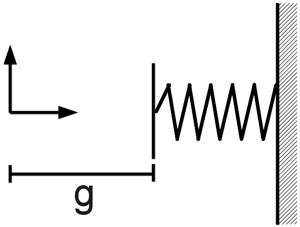
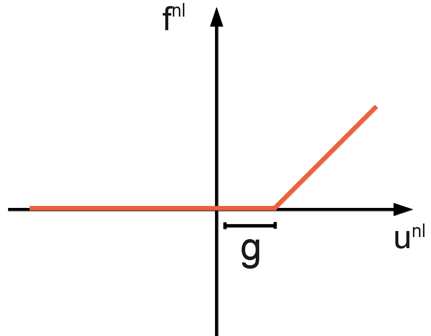
3.1. Unilateral contact

Unilateral contact nonlinearity, in its non-regular form, is written as:

\[\]

: label: eq-5

{mathrm {f}}} ^ {mathrm {nl}} (t) ={begin {array} {c}alpha ({u} ^ {mathit {nl}} (t) -g)mathit {si} -g)mathit {si} -g)mathit {si} -g)mathit {si} -g)mathit {si} -g)mathit {si} -g)mathit {si} -g)mathit {si} {u} {u} {u} {u} {u} {u} {u} {u} {u} {u} {u} {u} {u} {u} {u}} ^ {u} {u} {u}} ^ {u} {u} {u} {nl}} (t) ≤g,end {array}

where \(\alpha\) is the contact stiffness, \(g\) the gap between the structure node and the contact node. The proposed regularization is written in the implicit form

(3.4)\[ {\ mathrm {f}} ^ {\ mathrm {nl}} (t) (t) ({\ mathrm {f}} ^ {\ mathrm {nl}} (t) -\ alpha ({u} ^ {u} ^ {\ mathrm {nl}} ^ {\ mathit {nl}}} (t) -g)) -\ alpha\ eta =\ mathrm {0,} ^ {\ mathit {nl} ^ {\ mathit {nl}} (t) -g)) -\ alpha\ eta =\ mathrm {0,}\]

where \(\eta\) represents the regularization parameter.

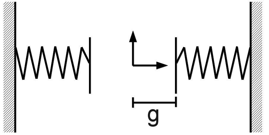
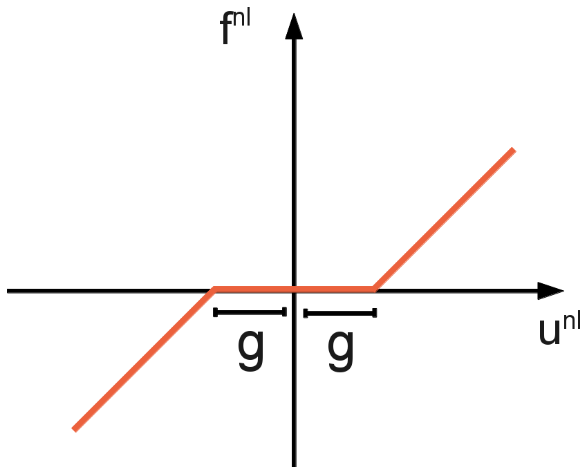
3.2. Bilateral contact

The nonlinearity of bilateral contact, in its non-regular form, is written as

(3.5)\[\begin{split} {\ mathrm {f}} ^ {\ mathrm {nl}} (t) =\ {\ begin {array} {c}\ alpha ({u} ^ {\ mathit {nl}} (t) -g)\ mathit {si} -g)\ mathit {si} -g)\ mathit {nl}} (t) age-g)\\\ 0\ mathit {si}} (t) -g)\ mathit {si} -g)\ mathit {si} -g)\ mathit {si} -g)\ mathit {si} -g)\ mathit {si} -g)\ mathit {si} -g)\ mathit {si} -g)\ mathit {si} -g)\ mathit {si} -g)\ mathit {si} -g mathit {nl}} (t)\ mid ≤g,\\\ alpha ({u} ^ {\ mathit {nl}} (t) +g)\ mathit {si} {u} ^ {\ mathit {nl}} ^ {\ mathit {nl}} ^ {\ mathit {nl}}} (t) ≤-g,\ end {array} ^ {\ mathit {nl}} ^ {\ mathit {nl}}} (t) ≤-g,\ end {array}\end{split}\]

where \(\alpha\) is the contact stiffness, \(g\) the gap between the structure node and the contact node. The proposed regularization is written in the following implicit form:

(3.6)\[ {f} ^ {\ mathit {nl}} (t) (t) ({f} ^ {f} ^ {f} ^ {f} ^ {\ mathit {nl}} (t) -g)) ({f} ^ {f} ^ {\ mathit {nl}} (t) ^ {\ mathit {nl}} (t) ^ {\ mathit {nl}} (t) +g)) ({f} ^ {f} ^ {f} ^ {f} ^ {f} ^ {f} ^ {f} ^ {f} ^ {f} ^ {f} ^ {f} ^ {f} ^ {f} ^ {f} ^ {f} ^ {f} ^ {f} ^ {f} ^ {f} ^ {f} ^ {f} ^ {f} ^ {f} ^\ alpha} ^ {2}\ eta {u} ^ {\ mathit {nl}} (t) =\ mathrm {0,}\]

where \(\eta\) represents the regularization parameter. We can rewrite it in quadratic form,

(3.7)\[\begin{split} \ {\ begin {array} {c} {\ alpha} {\ alpha} ^ {2} {2} {g} ^ {2} {f} ^ {\ mathit {nl}} (t) -\ eta {\ alpha} ^ {2} {u} {u} {u}} ^ {\ mathit {nl}} ^ {\ mathit {nl}} (t) =\ mathrm {0,}\\ z (t) - {({f} ^ {\ mathit {nl}}} (t) -\ alpha {u} ^ {\ mathit {nl}} (t))} ^ {2} =0))} ^ {2} =0. \ end {array}\end{split}\]

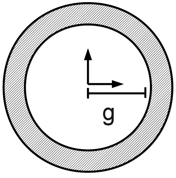
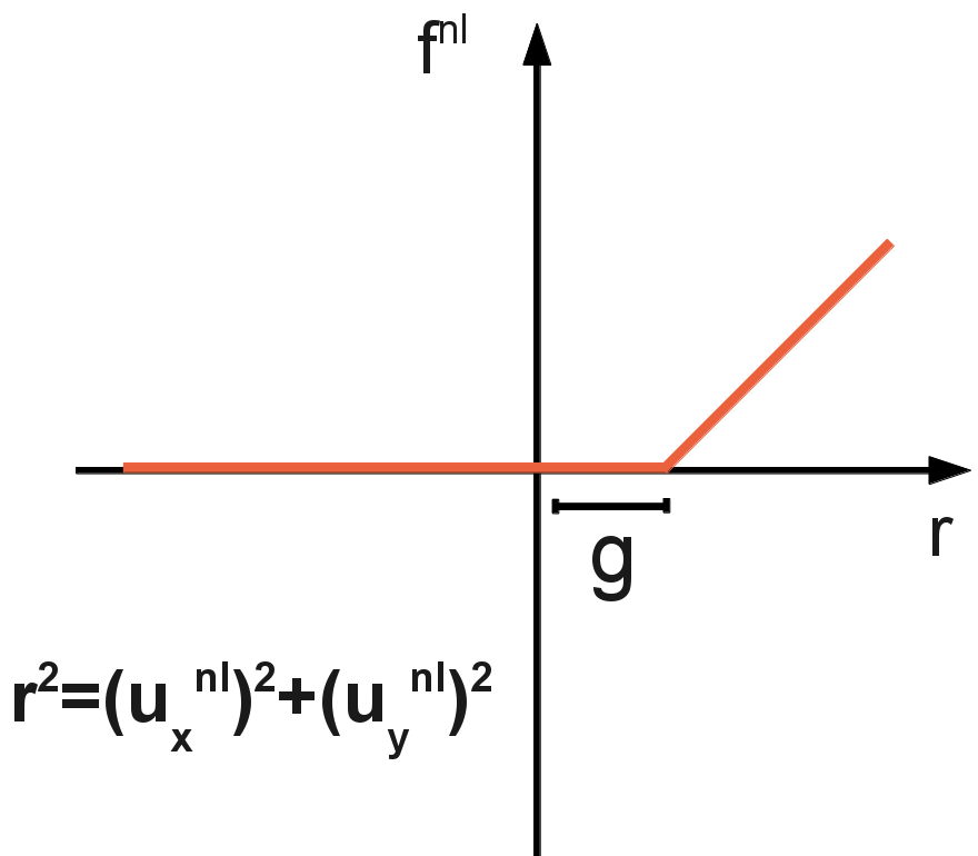
3.3. Ring contact

We enter \(z(t)\), the radial distance with respect to the equilibrium position \(({e}_{x},{e}_{y})\) of the shock node, whose current position is \(({u}_{x}^{\mathit{nl}},{u}_{y}^{\mathit{nl}})\). \(z(t)\) can be written

(3.8)\[ z (t) =\ sqrt {{\ left ({u} ({u} _ {x}} ^ {\ mathit {nl}}} (t) - {e} _ {x}\ right)} ^ {2} + {\ left ({u} _ {u} _ {u} _ {2}} + {u} _ {2}} + {u} _ {2}}\ mathrm {}}}\ mathrm {.}\]

The nonlinearity of annular contact, in its non-regular form, is written as

(3.9)\[\begin{split} {\ mathrm {f}} ^ {\ mathrm {nl}} (t) =\ {\ begin {array} {c}\ alpha (z (t) -g)\ mathit {si} z (t) >g,\\ 0\ mathrm {nl}}} (t) >g,\\ 0\ mathrm {nl}}} (t) >g,\\ 0\ mathrm {nl}}} (t) >g,\\ 0\ mathit {nl}}} (t) >g,\\ 0\ mathit {si} z (t) -g,\ end {array}\end{split}\]

where \(g\) refers to the radius of the ring (in other words the gap) and \(\alpha\) (\(\alpha >0\)) refers to the associated stiffness coefficient. By introducing the components \({f}_{x}^{\mathit{nl}}\) and \({f}_{y}^{\mathit{nl}}\) of the nonlinear force in the directions \(x\) and \(y\), the proposed regularization is written in the following implicit form

(3.10)\[\begin{split} \ {\ begin {array} {c} {\ mathrm {f}}} ^ {\ mathrm {f}}} (t)\ left ({\ mathrm {f}}} ^ {\ mathrm {nl}} (t) (t) -\ alpha (z (t) -g)}} ^ {g)} ^ {g)\ right) -\ alpha\ eta =\ mathrm {0,}\\ {z}} (t) -\ alpha (z (t) -g)\ right) -\ alpha (z (t) -g)\ right) -\ alpha\ eta =\ mathrm {0,}\\ {z} {nl}} (t) (t) -\ alpha (z (t) -g)\ right) -\ alpha\ (t) -g t) - {({u} _ {x} ^ {\ mathit {nl}} ^ {\ mathit {nl}}} (t) - {e} _ {x})} ^ {y} ^ {\ mathit {nl}} ^ {nl}} ^ (t) - {e} {nl}} (t) - {e} _ {nl}}} (t) - {e} _ {nl}}} (t) - {e} _ {nl}}} (t) - {e} _ {nl}}} (t) - {e} _ {y}} (t) - {e} _ {nl}}} (t) - {e} _ {nl}} (t) - {e} _ {nl}} (t) - {e} _ {nl}}} (t) mathit {nl}} (t) z (t) — {\ mathrm {f}}} ^ {\ mathrm {nl}} (t) {u} _ {x} ^ {\ mathit {nl}} (t) =\ mathrm {0,} =\ mathrm {0,}}\\ {f}} _ {y} ^ {\ mathit {nl}} ^ {\ mathit {nl}} ^ {\ mathit {nl}} ^ {\ mathit {nl}} ^ {\ mathit {nl}} ^ {\ mathit {nl}} ^ {\ mathit {nl}} ^ {\ mathit {nl}} ^ {\ mathit {nl}} ^ {\ mathit {nl}} ^ {\ mathit {nl}} (t) z (t) {f}} ^ {\ mathrm {nl}} (t) {u} _ {y} ^ {\ mathit {nl}} (t) =\ mathrm {0,}}\ end {array}\end{split}\]

where \(\eta\) represents the regularization parameter.