2. Contact relationships between two structures

Two relationships govern the contact between two structures:

• The one-sided contact relationship that expresses the non-interpenetrability between solid bodies,

• the friction relationship that governs the variation of tangential forces in contact. For the present developments, a simple relationship will be retained: Coulomb’s law of friction.

2.1. Unilateral contact relationship

Let’s say two structures \({\mathrm{\Omega }}_{1}\) and \({\mathrm{\Omega }}_{2}\). We note \({d}_{N}^{1/2}\) the normal distance between structures and \({F}_{N}^{1/2}\) the normal reaction force of \({\mathrm{\Omega }}_{1}\) out of \({\mathrm{\Omega }}_{2}\) (see figure).

Figure 2-1: Normal distance and normal reaction

The law of action and reaction requires:

(2.1)\[ {F} _ {N} ^ {1/2} =- {F} _ {N} ^ {2/1}\]

The conditions of unilateral contact, also called Signorin conditions (see [1]), are expressed as follows:

(2.2)\[\begin{split} \ {\ begin {array} {c} {d} _ {N} _ {N} ^ {1/2}\ ge 0\\ {F} _ {N} ^ {1/2}\ ge 0\\ {d} _ {N} _ {N} _ {N}} ^ {1/2} _ {1/2} _ {N} {D} _ {D} _ {N} {d} _ {N} _ {D} _ {N} _ {N} _ {N} ^ {1/2} _ {N} _ {N} ^ {1/2} _ {N} ^ {1/2} _ {N} ^ {1/2} _ {N\end{split}\]

Figure 2-2: Unilateral contact relationship graph

The graphic representation of the law of unilateral contact in the figure reflects a force-displacement relationship that is not differentiable. It is therefore not usable in a simple manner in a dynamic calculation algorithm.

If we restrict the study to the case of a tubular structure in the presence of an undeformable support, we note \({d}_{n}\left({d}_{n}={d}_{N}^{1/2}\right)\) the normal distance to the support, and \({F}_{n}\) the reaction of the latter (\({F}_{n}={F}_{N}^{2/1}=-{F}_{N}^{1/2}\) see figure).

Figure 2-3: Normal distance and normal reaction between a structure and a support

The expression of the conditions of normal contact, expressing the limitation of movements due to the support, is equivalent to:

(2.3)\[\begin{split} \ {\ begin {array} {c} {d} _ {n} _ {n}\ ge 0\\ {F} _ {n}\ ge 0\\ {d} _ {n} {F} _ {f} _ {n} _ {n} = 0\ end {array}\end{split}\]

2.2. Coulomb’s law of friction

Coulomb’s law expresses a limitation of the tangential force \({F}_{T}^{1/2}\) of tangential reaction of \({O}_{1}\) on \({O}_{2}\). Let \({\dot{u}}_{T}^{1/2}\) be the relative speed of \({\Omega }_{1}\) with respect to \({O}_{2}\) at a point of contact and let \(\mu\) be the Coulomb coefficient of friction, we have (see [1]):

\[\]

: label: eq-4

{begin {array} {c} s=Green {F} s=Green {F} _ {F} _ {N} ^ {1/2}le 0\existsmathrm {lambda}_ {1/2}le 0\existsmathrm {lambda}{lambda}text {lambda}text {lambda}text {such as} {dot {u}}} _ {T} ^ {1/2} =mathrm {lambda} F} _ {T} ^ {1/2}\mathrm {lambda}le 0\mathrm {lambda}mathrm {.} s=0end {array}

and the law of action and reaction:

\[\]

: label: eq-5

{F} _ {T} ^ {1/2} =- {F} _ {T} ^ {2/1}

The graphical representation of Coulomb’s law on the figure also reflects the non-differentiable nature of the law and is therefore not simple to use in a dynamic algorithm.

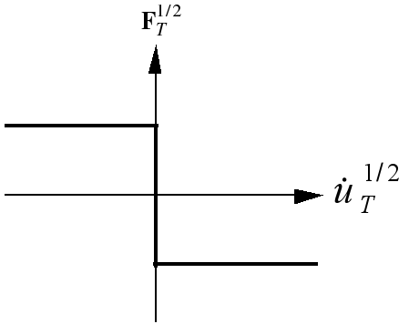
Figure 2-4: Graph of Coulomb’s law of friction

If the study is restricted to the case of a tubular structure in the presence of an undeformable support, only the tangential force \({F}_{T}^{2/1}={F}_{T}\) is used, the law of friction is expressed in the following way:

(2.4)\[\begin{split} \ {\ begin {array} {c} s=\ Green {F} s=\ Green {F} _ {F} s=\ Green -\ mathrm {\ mu} _ {n}\\ exists\ mathrm {\ lambda}\\ s=\ mathrm {\ lambda}\\ s=\ mathrm {\ lambda} {\ exists\ mathrm {\ lambda}\\ s=\\ mathrm {\ lambda}\ s=\\\ mathrm {\ lambda}\ le 0\\\ mathrm {\ lambda} s=0\ end {array}\end{split}\]

A common extension of Coulomb’s law, resulting from experience, consists in having two coefficients of friction: one for adhesion, noted \({\mu }_{s}\), the other for sliding, noted \({\mu }_{d}\), with \({\mu }_{s}>{\mu }_{d}\). We then have an adhesion phase \(\Vert {F}_{T}\Vert \le {\mathrm{\mu }}_{s}{F}_{n}\) and a sliding phase \(\Vert {F}_{T}\Vert ={\mathrm{\mu }}_{d}{F}_{n}\).