2. Theory

In this chapter, we use a seismic example to present the problem where we reason in an absolute frame of reference.

2.1. General principle

During an earthquake, the recorded signals are generally measured on a structure. Thus, when one wishes to study the dynamic behavior of this structure, the input signal is an unknown of the numerical model that must be determined (see FIG. 1).

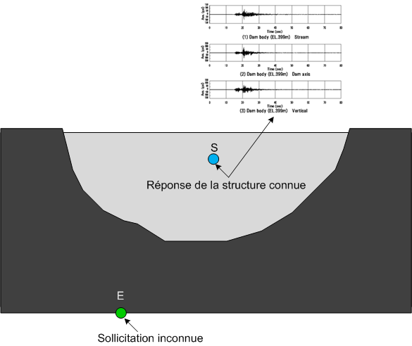
Figure 1 — Schematic representation of the problem

To reconstitute the input signal knowing the output signal (signal generally measured), we place ourselves in the frequency domain and we look for the transfer function \(\underline{\underline{H}}(\omega )\) between the two points of our system (see FIG. 2). The entry point corresponds to point E and the exit point to point S in FIG. 1.

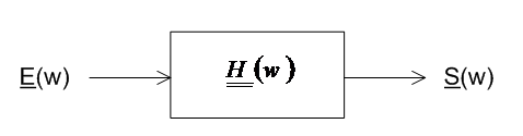
Figure 2 - Transfer function diagram

From several unidirectional dynamic calculations \({\gamma }_{i},\mathit{avec}i=x,y,z\), it is possible to access the transfer function by looking at the output \(\underline{S}(\omega )\) and the input \(\underline{E}(\omega )\).

Notes:

DeterminationInput and output signals must be of the same nature (ACCE / * ACCE or VITE/VITE or DEPL/DEPL).

It is recommended to use white noise signals in order to uniformly excite the structure over the entire frequency range.

Once the transfer function matrix is known, and knowing the desired output signal, it is possible to reconstitute the input signal to be injected into the dynamic model to find the output signal by solving the following matrix system:

\(\underline{{E}^{\mathit{absolu}}}(\omega )=\underline{\underline{{H}^{-1}}}(\omega )\underline{{S}^{\mathit{absolu}}}(\omega )\)

Where:

\(\underline{{S}^{\mathit{absolu}}}(\omega )\)	Vector containing the absolute accelerations measured at the exit point S of the structure during the earthquake
\(\underline{{E}^{\mathit{absolu}}}(\omega )\)	Vector containing the absolute accelerations to be applied to the input point E to find the absolute accelerations measured at the exit point S
\(\underline{\underline{{H}^{-1}}}(\omega )\)	Inverse transfer function matrix

2.2. Determination of the transfer function matrix \(\underline{\underline{H}}(\omega )\)

In this paragraph, we propose to present the equations that make it possible to determine the transfer function matrix \(\underline{\underline{H}}(\omega )\) in the three-dimensional case. To facilitate the definition of the problem, we treat the problem in terms of acceleration (the latter can also be treated in terms of displacement or speed).

Let \({E}_{i}^{\mathit{absolu}}\) and \({S}_{i}^{\mathit{absolu}}\) be the absolute accelerations calculated at the entry and exit points respectively. The aim is to solve the following system:

\(\underline{{S}^{\mathit{absolu}}}(\omega )=\underline{\underline{H}}(\omega )\underline{{E}^{\mathit{absolu}}}(\omega )\)

Where \(\{\begin{array}{c}{S}_{i}^{\mathit{absolu}}={S}_{i}^{\mathit{relatif}}+{\gamma }_{i},i=x,y,z\\ {E}_{i}^{\mathit{absolu}}={E}_{i}^{\mathit{relatif}}+{\gamma }_{i},i=x,y,z\end{array}\) and \(\underline{\underline{H}}(\omega )=\left(\begin{array}{ccc}{H}_{\mathit{xx}}& {H}_{\mathit{xy}}& {H}_{\mathit{xz}}\\ {H}_{\mathit{yx}}& {H}_{\mathit{yy}}& {H}_{\mathit{yz}}\\ {H}_{\mathit{zx}}& {H}_{\mathit{zy}}& {H}_{\mathit{zz}}\end{array}\right)\)

To determine the 9 unknowns of the problem, a system of 9 equations with 9 unknowns must be solved. This system is determined by carrying out three calculations with unidirectional loading in the x, y or z directions in order not to neglect the possible coupling between directions.

Harmonic calculation according to X

Let \(X\text{\_}{\mathit{sortie}}_{i}^{a},i=x,y,z\) be the absolute acceleration calculated at the exit point and \(X\text{\_}{\mathit{entree}}_{i}^{a},i=x,y,z\) the absolute acceleration calculated at the input point for a unidirectional excitation \({\gamma }_{x}\).

The system (E1) to be solved is as follows:

\((\mathit{E1})\text{}\{\begin{array}{c}X\text{\_}{\mathit{sortie}}_{x}^{a}={H}_{\mathit{xx}}X\text{\_}{\mathit{entree}}_{x}^{a}+{H}_{\mathit{xy}}X\text{\_}{\mathit{entree}}_{y}^{a}+{H}_{\mathit{xz}}X\text{\_}{\mathit{entree}}_{z}^{a}\\ X\text{\_}{\mathit{sortie}}_{y}^{a}={H}_{\mathit{yx}}X\text{\_}{\mathit{entree}}_{x}^{a}+{H}_{\mathit{yy}}X\text{\_}{\mathit{entree}}_{y}^{a}+{H}_{\mathit{yz}}X\text{\_}{\mathit{entree}}_{z}^{a}\\ X\text{\_}{\mathit{sortie}}_{z}^{a}={H}_{\mathit{zx}}X\text{\_}{\mathit{entree}}_{x}^{a}+{H}_{\mathit{zy}}X\text{\_}{\mathit{entree}}_{y}^{a}+{H}_{\mathit{zxz}}X\text{\_}{\mathit{entree}}_{z}^{a}\end{array}\)

Harmonic calculation according to Y

Let \(Y\text{\_}{\mathit{sortie}}_{i}^{a},i=x,y,z\) be the absolute acceleration calculated at the exit point and \(Y\text{\_}{\mathit{entree}}_{i}^{a},i=x,y,z\) the absolute acceleration calculated at the input point for a unidirectional excitation \({\gamma }_{y}\).

The system (E2) to be solved is as follows:

\((\mathit{E2})\text{}\{\begin{array}{c}Y\text{\_}{\mathit{sortie}}_{x}^{a}={H}_{\mathit{xx}}Y\text{\_}{\mathit{entree}}_{x}^{a}+{H}_{\mathit{xy}}Y\text{\_}{\mathit{entree}}_{y}^{a}+{H}_{\mathit{xz}}Y\text{\_}{\mathit{entree}}_{z}^{a}\\ Y\text{\_}{\mathit{sortie}}_{y}^{a}={H}_{\mathit{yx}}Y\text{\_}{\mathit{entree}}_{x}^{a}+{H}_{\mathit{yy}}Y\text{\_}{\mathit{entree}}_{y}^{a}+{H}_{\mathit{yz}}Y\text{\_}{\mathit{entree}}_{z}^{a}\\ Y\text{\_}{\mathit{sortie}}_{z}^{a}={H}_{\mathit{zx}}Y\text{\_}{\mathit{entree}}_{x}^{a}+{H}_{\mathit{zy}}Y\text{\_}{\mathit{entree}}_{y}^{a}+{H}_{\mathit{zxz}}Y\text{\_}{\mathit{entree}}_{z}^{a}\end{array}\)

Harmonic calculation according to Z

Let \(Z\text{\_}{\mathit{sortie}}_{i}^{a},i=x,y,z\) be the absolute acceleration calculated at the exit point and \(Z\text{\_}{\mathit{entree}}_{i}^{a},i=x,y,z\) the absolute acceleration calculated at the input point for a unidirectional excitation \({\gamma }_{z}\).

The system (E3) to be solved is as follows:

\((\mathit{E3})\text{}\{\begin{array}{c}Z\text{\_}{\mathit{sortie}}_{x}^{a}={H}_{\mathit{xx}}Z\text{\_}{\mathit{entree}}_{x}^{a}+{H}_{\mathit{xy}}Z\text{\_}{\mathit{entree}}_{y}^{a}+{H}_{\mathit{xz}}Z\text{\_}{\mathit{entree}}_{z}^{a}\\ Z\text{\_}{\mathit{sortie}}_{y}^{a}={H}_{\mathit{yx}}Z\text{\_}{\mathit{entree}}_{x}^{a}+{H}_{\mathit{yy}}Z\text{\_}{\mathit{entree}}_{y}^{a}+{H}_{\mathit{yz}}Z\text{\_}{\mathit{entree}}_{z}^{a}\\ Z\text{\_}{\mathit{sortie}}_{z}^{a}={H}_{\mathit{zx}}Z\text{\_}{\mathit{entree}}_{x}^{a}+{H}_{\mathit{zy}}Z\text{\_}{\mathit{entree}}_{y}^{a}+{H}_{\mathit{zxz}}Z\text{\_}{\mathit{entree}}_{z}^{a}\end{array}\)

By grouping the systems (E1), (E2) and (E3) together in the form of a global system (E), we obtain a system of 9 equations with 9 unknowns.

\((E)\text{}\left(\begin{array}{c}X\text{\_}{\mathit{sortie}}_{x}^{a}\\ X\text{\_}{\mathit{sortie}}_{y}^{a}\\ X\text{\_}{\mathit{sortie}}_{z}^{a}\\ Y\text{\_}{\mathit{sortie}}_{x}^{a}\\ Y\text{\_}{\mathit{sortie}}_{y}^{a}\\ Y\text{\_}{\mathit{sortie}}_{z}^{a}\\ Z\text{\_}{\mathit{sortie}}_{x}^{a}\\ Z\text{\_}{\mathit{sortie}}_{y}^{a}\\ Z\text{\_}{\mathit{sortie}}_{z}^{a}\end{array}\right)=\left(\begin{array}{ccccccccc}X\text{\_}{\mathit{entree}}_{x}^{a}& X\text{\_}{\mathit{entree}}_{y}^{a}& X\text{\_}{\mathit{entree}}_{z}^{a}& 0& 0& 0& 0& 0& 0\\ 0& 0& 0& X\text{\_}{\mathit{entree}}_{x}^{a}& X\text{\_}{\mathit{entree}}_{y}^{a}& X\text{\_}{\mathit{entree}}_{z}^{a}& 0& 0& 0\\ 0& 0& 0& 0& 0& 0& X\text{\_}{\mathit{entree}}_{x}^{a}& X\text{\_}{\mathit{entree}}_{y}^{a}& X\text{\_}{\mathit{entree}}_{z}^{a}\\ Y\text{\_}{\mathit{entree}}_{x}^{a}& Y\text{\_}{\mathit{entree}}_{y}^{a}& Y\text{\_}{\mathit{entree}}_{z}^{a}& 0& 0& 0& 0& 0& 0\\ 0& 0& 0& Y\text{\_}{\mathit{entree}}_{x}^{a}& Y\text{\_}{\mathit{entree}}_{y}^{a}& Y\text{\_}{\mathit{entree}}_{z}^{a}& 0& 0& 0\\ 0& 0& 0& 0& 0& 0& Y\text{\_}{\mathit{entree}}_{x}^{a}& Y\text{\_}{\mathit{entree}}_{y}^{a}& Y\text{\_}{\mathit{entree}}_{z}^{a}\\ Z\text{\_}{\mathit{entree}}_{x}^{a}& Z\text{\_}{\mathit{entree}}_{y}^{a}& Z\text{\_}{\mathit{entree}}_{z}^{a}& 0& 0& 0& 0& 0& 0\\ 0& 0& 0& Z\text{\_}{\mathit{entree}}_{x}^{a}& Z\text{\_}{\mathit{entree}}_{y}^{a}& Z\text{\_}{\mathit{entree}}_{z}^{a}& 0& 0& 0\\ 0& 0& 0& 0& 0& 0& Z\text{\_}{\mathit{entree}}_{x}^{a}& Z\text{\_}{\mathit{entree}}_{y}^{a}& Z\text{\_}{\mathit{entree}}_{z}^{a}\end{array}\right)\left(\begin{array}{c}{H}_{\mathit{xx}}\\ {H}_{\mathit{xy}}\\ {H}_{\mathit{xz}}\\ {H}_{\mathit{yx}}\\ {H}_{\mathit{yy}}\\ {H}_{\mathit{yz}}\\ {H}_{\mathit{zx}}\\ {H}_{\mathit{zy}}\\ {H}_{\mathit{zz}}\end{array}\right)\)

The terms \({H}_{\mathit{ij}}\) are then determined by inverting the matrix system (E) using the linear algebra resolution operators available in the Python numpy library,

2.3. Determining the signal to be reconstructed

When the terms \({H}_{\mathit{ij}}(\omega )\) of the transfer function matrix are known, it is possible to reconstitute the input signal knowing the output signal. To do this, simply solve the following matrix system:

\(\underline{{E}_{\mathit{reconstitué}}^{\mathit{absolu}}}(\omega )=\underline{\underline{{H}^{-1}}}(\omega )\underline{{S}_{\mathit{mesuré}}^{\mathit{absolu}}}(\omega )\)