3. Hysteretic damping model

3.1. Physical definition of hysteretic damping

For a sinusoidal excitation applied to an elasto-plastic structure or to an elastic structure with friction, the force-displacement curve reveals a positive work of the external force which corresponds to an energy dissipated in the structure, which can be represented as a first approximation as below:

In both cases the loss coefficient increases, generally with the amplitude of the cycle. For low values of the loss coefficient (less than \(\mathrm{0,2}\)), the shape of the cycle has no significant influence on the movement and can be likened to an ellipse [bib1].

In the particular case of a force-displacement relationship whose cycle is elliptical in shape, the expression for the loss coefficient is simple. For an applied force \(F\) and a displacement \(u\mathrm{=}{u}_{0}\text{cos}q\) the restoring force is \({\mathit{ku}}_{0}\text{cos}\theta\), \(k\) being the « classical » stiffness of the mechanical system, and the damping force \(\mathrm{-}{\mathit{hu}}_{0}\text{sin}\theta\), \(h\) being the stiffness out of phase by \(90°\), which leads to the behavioral relationship \(F\mathrm{=}{\mathit{ku}}_{0}\text{cos}\theta \mathrm{-}{\mathit{hu}}_{0}\text{sin}\theta\).

The energies, dissipated during a cycle and maximum potential, are:

(3.1)\[ {E} _ {d} ^ {\ text {cycle}} = {\ int}} = {\ int}} _ {\ int} _ {\ int} _ {0}\ text {sin}\ theta d\ left ({u} _ {0}\ text {u} _ {0}\ text {cos}\ theta\ right) =\ pi {\ mathit {hu}}} _ {0}\ left ({u} _ left ({u} _ left ({u} _ {0} _ {0} _ {0} _ {0} _ {0} _ {0} _ {0} _ {0} _ {0} _ {0} _ {0} _ {0} _ {0} _ {0} _ {2}}\]

and:

(3.2)\[ {E} _ {p} ^ {\ text {max}} = {\ text {max}}} = {\ int}} _ {\ text {max}}} = {0}\ text {cos}\ theta d\ left ({u} _ {0}}\ {0}\ text {cos}\ theta\ right) =\ frac {{\ mathit {ku}}} _ {0}\ left ({u} _ {left) ({u} _ {0} _ {0} _ {0} _ {0} _ {0} _ {0} _ {0} _ {0} _ {0} _ {0} _ {0} _ {0} _ {0} _ {0} _ {0} _ {0} _ {0} _ {0} _ {0} _ {2}} 2}\]

Hence the loss coefficient:

(3.3)\[ \ eta\ mathrm {=}\ frac {\ frac {\ pi {\ mathit {hu}}} _ {0} ^ {2}} {2\ pi\ frac {{\ mathit {ku}}} _ {0}} ^ {2}} {2}}\ mathrm {=}\ frac {ku}}} _ {0}} ^ {2}}\]

For a sine cycle \(\theta =\omegat\), the hysteretic damping coefficient \(\eta =\frac{h}{k}\) is independent of \(\omega\). It can be determined from a test under harmonic cyclic loading.

3.2. Harmonic oscillator with hysteretic damping

The hysteretic damping model can be used to treat the harmonic responses of structures with viscoelastic materials.

The energy dissipated per cycle in the form \({E}_{d}^{\text{cycle}}={\int }_{0}^{2\pi }\sigma d\epsilon\) makes it possible to demonstrate a complex Young’s modulus \({E}^{\text{*}}\) from the stress-strain relationship of a viscoelastic material \(\sigma ={\sigma }_{0}{e}^{j\omega t}\) and \(\epsilon ={\epsilon }_{0}{e}^{j\left(\omega t-\phi \right)}\) where \({\sigma }_{0}\) and \({\epsilon }_{0}\) are the amplitudes and \(\varphi\) the phase:

(3.4)\[ {E} ^ {\ text {*}}} =\ frac {\ sigma} {\ sigma} {\ epsilon} =\ left (\ frac {{\ sigma} _ {\ epsilon} _ {0}}}\ right) {e}}\ right) {e}} {e}} {e}} {e}} {e} ^ {\ sigma} =\ left (\ frac {{\ sigma} _ {0}}} {{\ epsilon} _ {0}} {{\ epsilon}}\ right) {e}} {e}} {e}} {e}} {e}} {e} ^ {\ sigma} =\ left (\ frac {{\ sigma} _ {0}}} {{\ epsilon} _ {0}}}\ right)\ left (\ text {cos}\ phi}\ phi +j\ text {sin}\ phi\ right)\]

By noting \({E}_{1}=\left(\frac{{\sigma }_{0}}{{\epsilon }_{0}}\right)\text{cos}\phi\) the real part and \({E}_{2}=\left(\frac{{\mathrm{\sigma }}_{0}}{{\mathrm{\epsilon }}_{0}}\right)\text{sin}\mathrm{\phi }\) the imaginary part we get:

(3.5)\[ {E} ^ {\ text {*}}} = {E} _ {1}} + {\ mathit {jE}} _ {2} = {E} _ {1}\ left (1+j\ eta\ right)\]

with \(\eta =\frac{{E}_{1}}{{E}_{2}}=\text{tg}\phi\) where \(\phi\) is also called the loss angle.

The classical analysis of equation () only makes sense, with a hysteretic damping model, for harmonic excitation \(f(t)={f}_{0}{e}^{j\omegat }\) which leads to the equation:

(3.6)\[ m\ ddot {u} +k\ left (1+j\ eta\ right) u=m\ ddot {u} +\ left (k+\ mathit {jh}\ right) u= {f} _ {0} _ {0} {0} {0} {e} {e} ^ {j\ omega t}\]

where the real part of the displacement \(u\) represents the movement of the mass and \(h=k\eta\).

As before [§ 2.2], the harmonic response can be written, with the reduced pulse \(\mathrm{\lambda }=\frac{\omega }{{\omega }_{0}}\), in the following form:

(3.7)\[ \ frac {{\ mathit {ku}} _ {0}} {0}} {{0}}} =\ frac {1} {1} {1- {\ lambda} ^ {2} +j\ eta} = {H}} = {H}\ left (j\ omega\ right)\]

where \({H}_{h}(j\omega )\) is the complex transfer function of a simple oscillator with hysteretic damping.

The answer modulus:math: frac {{u} _ {{u} _ {0}} {{0}}} {{u}} _frac {{mathit {ku}} _ {0}} {{0}}} {{f}}} {{f} _ {0}}} =| {H} _ {0}}} =| {H} _ {h}}left (jomegaright) |=frac {1} {sqrt {{right) |=frac {1} {sqrt {{left (1- {lambda} ^ {2}right)} ^ {2}right)} ^ {2}}}} shows dynamic amplification in relation to the static response, which is maximum for:math: lambda =1 and gives the maximum displacement value:math:frac {{u} _ {0text {max}}} {{u}}} {lambda =1 and gives the maximum displacement value:math: lambda =1 and gives the value of the maximum displacement:math:`frac {{u}} _ {text {st}}} =frac {1} {eta} =frac {1} {2xi} `.

In conclusion, the reduced damping associated with hysteretic damping is:

(3.8)\[ \ xi =\ frac {\ eta} {2} =\ frac {h} {2k} =\ frac {h} {2m {\ omega} _ {0}} ^ {2}}\]

3.3. Focus on linear viscoelasticity

Linear viscoelastic materials have laws of behavior of the type:

(3.9)\[ L\ sigma =M\]

where \(M\) and \(L\) are linear differential operators of the time variable, i.e. of the type \(L=\sum {l}_{k}{\partial }_{t}^{{\alpha }_{k}}\) where \({l}_{k}\) are real tensors and \({\alpha }_{k}\) are the potentially non-integer orders of derivation.

To calculate the movement at a given moment \(t\), you need to know the dynamics of the previous moments: in this sense, the movement at time \(t\) depends on its history. While integer time derivative models require knowledge of the speed, acceleration, or higher orders of motion to calculate the forces at a given point in time, fractional order models need the full history of motion. Indeed, fractional derivatives have the characteristic of being non-local: for example the Grunwald-Letnikov derivative of \(f\) in \(x\) of order \(\alpha\) is defined as the limit when \(h\to 0\) of the finite difference:

(3.10)\[\begin{split} \ frac {1} {{h} ^ {\ alpha}}}\ sum _ {k=0}} ^ {\ mathrm {\ infty}} {(-1)} ^ {k}\ left (\ begin {array}\ left (\ begin {array} {c} {c}}\ c}\ c}\ c}\ c}\ sum _ {\ alpha}}}\ sum _ {k=0} ^ {\ infty}}} {(-1)} ^ {k}\ left (\ begin {array} {c} {c}}\ c}\ c}\ left (\ begin {array} {c}}\ c}\ c}\ alpha\\ k}\ left\end{split}\]

so each point \(y<x\) is taken into account for the calculation of this derivative.

The temporal calculation of a viscoelastic material, although conceptually simple, is complicated to implement on industrial application cases. The evaluation of the law of behavior requires being able to access quickly and a large number of subsequent calculation moments.

Harmonic calculation is very simple to perform, in fact the law of behavior \(L\sigma =M\epsilon\) becomes:

(3.11)\[ \ sigma = {H} _ {c} (\ omega)\ epsilon\]

where \({H}_{c}(\omega )\) is a Hooke tensor with complex, frequency-dependent values. Two families of rheological models compete for modeling the elastic modules of the Hooke tensor:

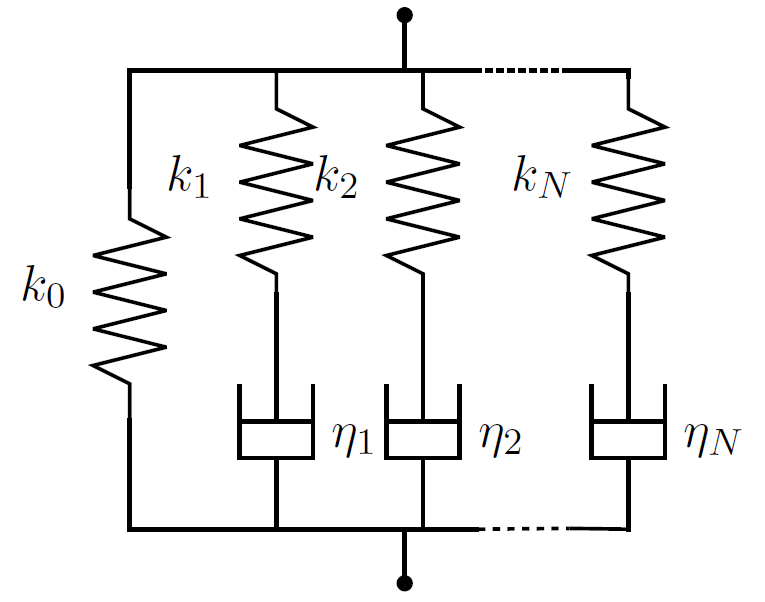
• Compound models: the polymers forming the viscoelastic material are modelled as a series or parallel arrangement of an elementary pattern composed of shock absorbers and pistons.

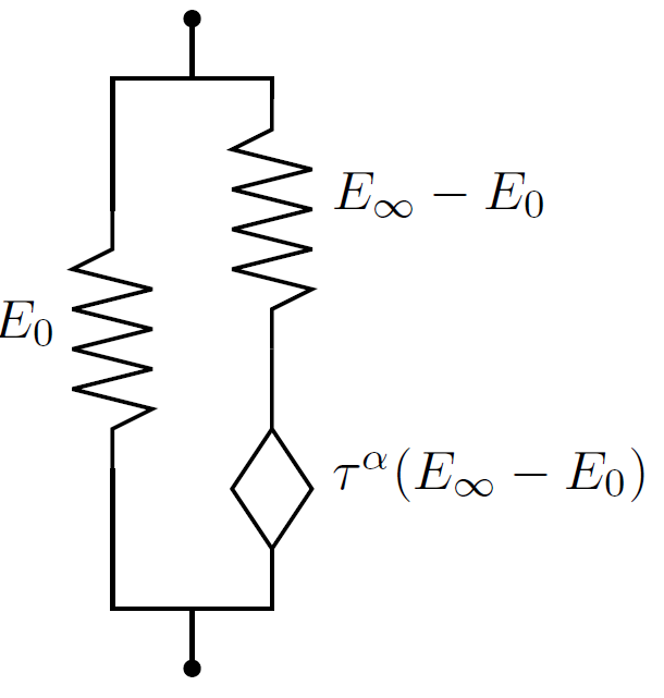
• Fractional models: polymer chains are modelled in one block by an elementary pattern including springs, pistons and « pistors » of alpha order (a pistor is an element that has associated a deformation \(u\) \({\partial }_{t}^{\alpha }u\) associates)

Examples of models:

Model	Maxwell Range	Fractional Zener
Variation with \(\omega\) of the modules	\({E}^{\text{*}}(\omega )=\sum _{k=1}^{N}{E}_{k}\frac{j{\omega }_{k}{\eta }_{k}}{{E}_{k}+j{\omega }_{k}{\eta }_{k}}\)	\({E}^{\text{*}}(\omega )=\frac{{E}_{0}+{E}_{\mathrm{\infty }}{(j\omega \tau )}^{\alpha }}{1+{(j\omega \tau )}^{\alpha }}\)
Diagram

Compound models generally need a number of \(N\) terms greater than \(15\), the number of coefficients to be determined by tests can be important. While a fractional Zener model only needs four numbers to stick to the experimental curves.

A viscoelastic material is therefore a material which, in the frequency domain, follows a Hooke’s law whose elasticity modules are complex and dependent on frequency. The coefficients of the model for each elasticity module (\(E\), \(G\),,,, \(\nu\), \(K\),…) are measured by specific tests at various frequencies.

For example, an isotropic viscoelastic material modelled by a fractional Zener law has the law of behavior:

(3.12)\[ \ sigma =2\ frac {{G} _ {0} _ {0} + {0} + {0} + {G} + {G} + {G} + {G}}} ^ {{\ alpha} _ {G}}} {G}}} {G}}} {1+ {(j\ omega {\ tau} _ {G}})} ^ {{\ alpha} _ {G}}}} ^ {\ alpha} _ {G}}}} ^ {\ alpha} _ {G}}}} ^ {\ alpha} _ {G}}}} ^ {\ alpha} _ {G}}} (\ epsilon -\ frac {1} {3}\ mathit {Tr} ()\ mathit {Id}) +\ frac {{K} _ {0} + {K} _ {\ mathrm {\ infty}}} {(j\ omega {\ tau}}} {{K}}} {(j\ omega {\ infty}}}} {(j\ omega {\ infty}}}} {(j\ omega {\ infty}}}} {(j\ omega {\ infty}}}} {(j\ omega {\ infty}}}} {(j\ omega {\ infty}}}} {(j\ omega {\ tau}}}} {(j\ omega {\ tau}}}} {(j\ omega {\ tau}}}} {(j\ omega)} ^ {{\ alpha} _ {K}}}}\ mathit {Tr} (\ epsilon)\ mathit {Id}\]

This material must therefore be characterized in frequency by determining the two quadruplets \(({G}_{\mathrm{0,}}{G}_{\mathrm{\infty }},{\alpha }_{G},{\tau }_{G})\) and \(({K}_{\mathrm{0,}}{K}_{\mathrm{\infty }},{\alpha }_{K},{\tau }_{K})\).