5. Structure analysis with damping#
The models presented are not easily generalizable to the various structural analyses.
**Note: The two models do not have the same linear analysis domain. Viscous damping can be used in transient or harmonic analysis and* hysteretic damping can only be used in harmonic analysis.
The modeling options allow the definition of global damping for the structure and damping localized on cells or groups of cells.
5.1. Overall amortization of the structure#
In the absence of sufficient information on the components and connections that create energy dissipation, a common modeling consists in building a global damping matrix.
5.1.1. Global proportional viscous damping (Rayleigh)#
We place ourselves within the framework of classical equations for the dynamics of linear structures:
: label: eq-20
Mddot {U} +Cdot {U} +mathrm {KU} =F (t)
The concept of Rayleigh damping makes it possible to define damping matrix \(C\) as a linear combination of stiffness and mass matrices:
: label: eq-21
C=alpha K+beta M
Advantages:
easy to implement using operators DEFI_MATERIAU [U4.43.01] and ASSEMBLAGE (OPTION =” AMOR_MECA “). It is also possible to use the operator COMB_MATR_ASSE [U4.53.01], after assembling the stiffness and mass matrices with real coefficients;
useful for validating resolution algorithms;
historically, its success is linked to methods of transient analysis by modal recombination based on real eigenmodes. The orthogonality properties of real eigenmodes (solutions of the problem to eigenvalues \(\left(K-{\omega }^{2}M\right)\phi =0\)) result in the simultaneous diagonalization in the transition to generalized modal coordinates of \({\phi }^{T}K\phi\) and \({\phi }^{T}M\phi\). Rayleigh damping is a sufficient condition to diagonalize \({\phi }^{T}C\phi\). The system of modal equations \(\ddot{q}+\frac{{\phi }^{T}C\phi }{{\phi }^{T}M\phi }\dot{q}+{\omega }^{2}q=\frac{{\phi }^{T}}{{\phi }^{T}M\phi }F(t)\) then becomes diagonal:
Disadvantages:
This modeling does not make it possible to represent the heterogeneity of the structure in relation to damping.
The depreciation actually introduced in the model depends heavily on the identification of the coefficients \(\alpha\) and \(\beta\) Cf. [§ 5.1.2].
5.1.2. Influence of proportional damping coefficients#
Three simple identification cases are presented here to illustrate the effects induced by this modeling:
damping proportional to inertia characteristics: \(\mathrm{\alpha }=0\) and \(\beta\)
This case has been widely used in direct transient resolution: if the mass matrix is diagonal, the damping matrix is still diagonal and the gain in memory space is obvious. The coefficient \(\beta\) can be identified with the experimental reduced damping \({\xi }_{1}\) of the eigenmode \(\left({\phi }_{1},{\omega }_{1}\right)\) which contributes the most to the response, hence \(\beta =2{\xi }_{1}{\omega }_{1}\). For any other pulsation a reduced modal damping \(\mathrm{\xi }=\mathrm{\beta }\frac{{\mathrm{\omega }}_{1}}{\mathrm{\omega }}\) is obtained. High modes \(\omega \text{>>}{\omega }_{i}\) will be damped very little and low frequency modes \(\omega <{\omega }_{1}\) too damped.

damping proportional to stiffness characteristics: \(\mathrm{\alpha }\) and \(\beta =0\)
The coefficient \(\alpha\) can be identified, as previously, from \({\xi }_{2}\) associated with the mode \(\left({\mathrm{\phi }}_{2},{\mathrm{\omega }}_{2}\right)\), from where \(\alpha =2{\xi }_{2}{\omega }_{2}\). For any other pulsation a reduced modal damping \(\xi =\alpha \frac{\omega }{{\omega }_{2}}\) is obtained. High modes \(\omega \text{>>}{\omega }_{2}\) are very damped.

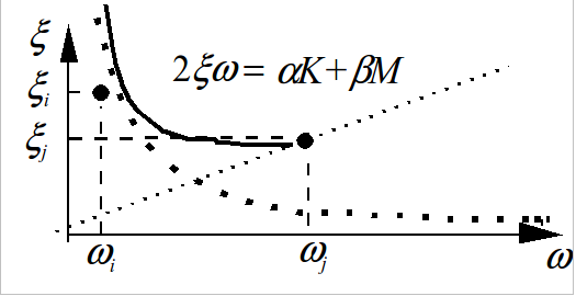
full proportional damping: \(\mathrm{\alpha }\) and \(\beta\)
From an identification on two independent modes \(({\varphi }_{1},{\omega }_{1})\) and \(({\varphi }_{2},{\omega }_{2})\), for any other pulsation, a reduced modal damping \(\mathrm{\xi }=\frac{1}{2}\left(\mathrm{\alpha }\mathrm{\omega }+\frac{\mathrm{\beta }}{\mathrm{\omega }}\right)={\mathrm{\xi }}_{1}\frac{\mathrm{\omega }}{{\mathrm{\omega }}_{1}}+{\mathrm{\xi }}_{2}\frac{{\mathrm{\omega }}_{2}}{\mathrm{\omega }}\) is obtained.
In the interval \(\left[{\omega }_{1},{\omega }_{2}\right]\), the variation in the reduced damping is low and outside this we find the addition of the previous disadvantages: the modes outside the interval are too damped.
In none of the above cases, it will be possible to reproduce a hypothesis of equal modal damping for all modes. Methods have been invented to reach this objective [bib1].
5.1.3. Global hysteretic damping#
The generalization of the simple oscillator equation with hysteretic damping leads to the system of complex equations where \(F\left(\mathrm{\Omega }\right)\) is a harmonic excitation.
Knowing the real stiffness matrix, it is possible to build a hysteretic damping matrix \({K}_{h}=j\eta K\), with an overall loss coefficient \(\eta\).
As before in resolution by modal recombination, from a base of real eigenmodes, we obtain \({\phi }^{T}M\phi \ddot{q}+j{\phi }^{T}{K}_{h}\phi q+{\phi }^{T}K\phi q={\phi }^{T}F(t)\) where the generalized hysteretic damping matrix is diagonal \({\phi }^{T}{K}_{h}\phi \text{=}\left[\text{diag}\eta {\gamma }_{i}\right]\), like the generalized stiffness matrix \({\phi }^{T}K\phi =\left[\text{diag}{\gamma }_{i}\right]\).
According to the definition of reduced damping, modal damping is constant for all modes hence \(\xi =\frac{\eta }{2}\).
Advantages:
easy to implement using operators DEFI_MATERIAU [U4.43.01] and ASSEMBLAGE (OPTION =” RIGI_MECA_HYST “) [U4.61.21]. It is also possible to proceed using the operator COMB_MATR_ASSE [U4.53.01], after assembling the stiffness matrix;
very useful for validating resolution algorithms;
The depreciation actually introduced in the model is constant for all modes of the structure, as required by building regulations.
Disadvantages:
this modeling is poorly suited for industrial studies, as it does not make it possible to represent the heterogeneity of the structure in relation to damping;
only harmonic analysis (in complex) is possible.
5.1.4. Viscoelastic hysteretic damping#
The structure is damped by a viscoelastic material, the harmonic calculation then aims to solve the equation:
The determination of complex modes is currently only possible by using DYNA_VISCO [U4.53.04] which makes it possible to calculate the modes in air of an isotropic viscoelastic material whose Poisson’s ratio is real.
Advantages:
easy to implement using operators DEFI_MATERIAU [U4.43.01] and ASSEMBLAGE (OPTION =” RIGI_MECA_HYST “) [U4.61.21];
amortization is physical.
Disadvantages:
only harmonic analysis (in complex) is possible.
5.2. Localized amortization#
For analyses requiring modeling representing the heterogeneity of the structure, it is possible to assign damping characteristics located on the cells of the structure, in fact on elements of the model.
5.2.1. Damping elements#
It is possible to apply discrete damping elements:
on POI1 cells: the damping is linked to the movement (respectively the speed) of the support node,
on cells SEG2: the damping is linked to the relative displacement (respectively the relative speed) of the two connected nodes.
The operator AFFE_CARA_ELEM [U4.24.01] allows you to define for each discrete element:
a \({a}_{\text{discret}}\) viscous damping matrix whose terms are assigned to the different degrees of freedom of the nodes concerned; several ways of describing the matrix are available.
a hysteretic loss coefficient \({\eta }_{\text{discret}}\) multiplying the stiffness matrix of the discrete element assigned to the support mesh.
5.2.2. Depreciation assigned to any type of finite element#
The elastic material assigned to any finite element can be defined with damping parameters by the operator DEFI_MATERIAU [U4.23.01].
Proportional viscous damping with two Rayleigh parameters \(\alpha\) and \(\beta\).
AMOR_BETA = \(\beta\)
For all types of finite elements (continuous, structural or discrete media), it is possible to calculate the real elementary matrices corresponding to the calculation option “AMOR_MECA”, after having calculated the elementary matrices corresponding to the calculation options” RIGI_MECA “and” MASS_MECA “.
The elementary matrix of the element \(i\) affected by the material \({\alpha }_{j},{\beta }_{j}\) is then of the form:
for a finite element:
for a discrete element:
Hysteretic damping with a coefficient of \(\eta\)
For all types of finite elements (continuous, structural or discrete media), it is possible to calculate the complex elementary matrices corresponding to the calculation option “RIGI_MECA_HYST”, after having calculated the elementary matrices corresponding to the calculation options” RIGI_MECA “.
The elementary matrix of the element \(i\) affected by the material \({\alpha }_{j},{\beta }_{j}\) is then of the form:
for a finite element:
: label: eq-27
{k} _ {text {elem}, i}} ^ {text {*}} = {k} _ {text {elem}, i}left (1+j {eta}} _ {j}right)
for a discrete element:
: label: eq-28
{k} _ {text {elem}, i}} ^ {text {*}}} = {k} _ {text {elem}, i}left (1+j {eta}} _ {text {discrete}, i}right)
5.2.3. Construction of the damping matrix#
The assembly of the elementary damping matrices is obtained with the usual operator ASSE_MATRICE [U4.42.02] or by the command ASSEMBLAGE [U4.31.02]. The same numbering and the same storage mode should be used as for the stiffness and mass matrices (operator NUME_DDL [U4.42.01]).
Note: the amortization matrix obtained is not proportional \(C\ne \alpha K+\beta M\) or \({K}_{h}\ne j\eta K\).