3. The diagram WILSON - \(\theta\) [bib1]#
3.1. Presentation of the diagram#
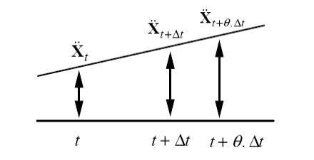
In what follows, it will be assumed that solids are linear elastic. This method assumes that the acceleration is linear between \(t\) and \(t+\theta \text{.}\Delta t\):
\({\ddot{\mathrm{X}}}_{\mathrm{t}+\mathrm{\tau }}={\ddot{\mathrm{X}}}_{t}+\frac{\tau }{\theta \mathrm{\Delta }t}\text{.}\text{}\left({\ddot{\mathrm{X}}}_{t\text{+}\theta \text{.}\mathrm{\Delta }t}-{\ddot{\mathrm{X}}}_{t}\right)\) eq 3.1-1
By integrating [éq3.1-1] as a function of the variable \(t\), we get:
\({\dot{\mathrm{X}}}_{t\text{+}\tau }={\dot{\mathrm{X}}}_{t}+\tau {\ddot{\mathrm{X}}}_{t}+\frac{{\tau }^{2}}{2\theta \mathrm{\Delta }t}\left({\ddot{\mathrm{X}}}_{t\text{+}\theta \text{.}\mathrm{\Delta }t}-{\ddot{\mathrm{X}}}_{t}\right)\) eq 3.1-2
\({\mathrm{X}}_{t+\tau }=\text{}{\mathrm{X}}_{t}+\tau {\dot{\mathrm{X}}}_{t}+\frac{{\tau }^{2}}{2}\ddot{\mathrm{X}}+\frac{{\tau }^{3}}{6\theta \mathrm{\Delta }t}\left({\ddot{\mathrm{X}}}_{t\text{+}\theta \text{.}\mathrm{\Delta }t}-{\ddot{\mathrm{X}}}_{t}\right)\) eq 3.1-3
We write the equilibrium equations at time \(t+\theta \text{.}\Delta t\) with \(\theta \ge 1\):
\(M\text{.}{\ddot{X}}_{t+\theta \Delta t}+\text{}C\text{.}{\dot{X}}_{t+\theta \Delta t}+\text{}K\text{.}{X}_{t+\theta \Delta t}\text{}=\text{}{R}_{t+\theta \Delta t}\) eq 3.1-4
by expressing \({\dot{X}}_{t+\theta \text{.}\Delta t }\) and \({\ddot{X}}_{t+\theta \text{.}\Delta t }\) according to \({\ddot{X}}_{t+\theta \text{.}\Delta t }\) and \({X}_{t}\), \({\dot{X}}_{t}\) and \({\ddot{X}}_{t}\) by the system [éq3.1‑2], [éq3.1-3], and substituting in [éq3.1-4], it comes:
\(\tilde{K}\text{.}{X}_{t+\theta \text{.}\Delta t }=\tilde{R}\)
where
\(\tilde{K}=K+\frac{3}{(\theta \text{.}\Delta t)}\text{.}C+\frac{6}{{(\theta \text{.}\Delta t)}^{2}}\text{.}M\)
\(\tilde{R}={R}_{t}+\theta \text{.}({R}_{t+\Delta t}-{R}_{t})+M\text{.}({a}_{0}\text{.}{X}_{t}+{a}_{2}\text{.}{\dot{X}}_{t}+2\text{.}{\ddot{X}}_{t})+C\text{.}({a}_{1}\text{.}{X}_{t}+2\text{.}{\dot{X}}_{t}+{a}_{3}\text{.}{\ddot{X}}_{t})\)
\(\begin{array}{ccccccc}{a}_{0}=\frac{6}{{(\theta \text{.}\Delta t )}^{2}}& & {a}_{1}=\frac{3}{(\theta \text{.}\Delta t )}& & {a}_{2}=2\text{.}{a}_{1}& & {a}_{3}=\frac{\theta \text{.}\Delta t }{2}\end{array}\)
We go back to movements, speeds and accelerations at step \(t+\Delta t\) by relationships:
\(\begin{array}{c}{\ddot{X}}_{t\text{+}\Delta t}={a}_{4}\text{.}({X}_{t\text{+}\theta \text{.}\Delta t}-{X}_{t})+{a}_{5}\text{.}{\dot{X}}_{t}+{a}_{6}\text{.}{\ddot{X}}_{t}\\ {\dot{X}}_{t\text{+}\Delta t}={\dot{X}}_{t}+{a}_{7}\text{.}({\ddot{X}}_{t+\Delta t}+{\ddot{X}}_{t})\\ {X}_{t\text{+}\Delta t}={X}_{t}+\Delta t\text{.}{\dot{X}}_{t}+{a}_{8}\text{.}({\ddot{X}}_{t\text{+}\Delta t}+2\text{.}{\ddot{X}}_{t})\end{array}\)
\(\begin{array}{ccccccccc}{a}_{4}=\frac{{a}_{0}}{\theta }& & {a}_{5}=\frac{-{a}_{2}}{\theta }& & {a}_{6}=1-\frac{3}{\theta }& & {a}_{7}=\frac{\Delta t }{2}& & {a}_{8}=\frac{\Delta {t}^{2}}{6}\end{array}\)
3.2. Complete algorithm for method WILSON - \(\theta\)#
a) initialization:
initial conditions \({X}_{0},{\dot{X}}_{0}\) and \({\ddot{X}}_{0}\)
choice of \(\Delta t\) and \(\theta\) and calculation of the coefficients \({a}_{1}\),… \({a}_{8}\) (see above)
assemble the \(K\) stiffness and \(M\) mass matrices
form the effective stiffness matrix \(\tilde{K}=K+{a}_{0}\text{.}M+{a}_{1}\text{.}C\)
Factorize \(\tilde{K}\)
b) at each time step:
calculate the actual load \(\tilde{R}\) |
|
\(\tilde{R}={R}_{t}+\theta \text{.}({R}_{t\text{+}\Delta t}-{R}_{t})+M\text{.}({a}_{0}\text{.}{X}_{t}+{a}_{2}\text{.}{\dot{X}}_{t}+2\text{.}{\ddot{X}}_{t})+C\text{.}({a}_{1}\text{.}{X}_{t}+2\text{.}{\dot{X}}_{t}+{a}_{3}\text{.}{\ddot{X}}_{t})\) |
|
solve \(\tilde{K}\text{.}{X}_{t+\theta \text{.}\Delta t}=\tilde{R}\) |
|
calculate the movements at time \(t+\Delta t\) \(\begin{array}{c}{\ddot{X}}_{t\text{+}\Delta t}={a}_{4}\text{.}({X}_{t\text{+}\theta \text{.}\Delta t}-{X}_{t})+{a}_{5}\text{.}{\dot{X}}_{t}+{a}_{6}\text{.}{\ddot{X}}_{t}\\ {\dot{X}}_{t\text{+}\Delta t}={\dot{X}}_{t}+{a}_{7}\text{.}({\ddot{X}}_{t\text{+}\Delta t}+{\ddot{X}}_{t})\\ {X}_{t\text{+}\Delta t}={X}_{t}+\Delta t\text{.}{\dot{X}}_{t}+{a}_{8}\text{.}({\ddot{X}}_{t\text{+}\Delta t}+2\text{.}{\ddot{X}}_{t})\end{array}\) |
|
calculation of the next time step: back to the beginning |
3.3. Stability condition for diagram WILSON - \(\theta\)#
The method is unconditionally stable for WILSON - \(\theta\) > 1.37, with a commonly used value for \(\theta\) being 1.4. In addition, the method has digital dissipation for \(\theta >1\), all the more important as \(\theta\) increases; but it can also generate parasitic oscillating amplifications at high frequencies.
The keyword factor WILSON makes it possible to specify the use of this algorithm and the choice of the value of \(\theta\). By default, the value of \(\theta\) is set to 1.4.
For the value of \(\theta\) equal to 1, the Wilson- \(\theta\) scheme is equal to the so-called « linear acceleration » schema, i.e. the Newmark schema with \(\gamma =1/2;\beta =1/6\) which is conditionally stable.