5. Numerical amortization of implicit schemes

The numerical advantage of direct implicit integration schemes lies in the fact that the time step can be substantially large compared to the smallest specific period of the system without risking causing instability in the results.

However, if the content of the response lies in a set of natural modes, the highest of which has a natural frequency \({F}_{\mathrm{max}}\), we will still have to respect a criterion on the time step of the form:

\(\mathrm{\Delta }t<\frac{0.1}{{F}_{\text{max}}}\text{à}\frac{0.01}{{F}_{\text{max}}}\)

For modes with a specific period in the order of a time step or less than a time step, the integration algorithms introduce a strong damping that contributes to erasing the contribution of these high modes.

We can see on the graph below the decrease in amplitude of a system to one degree of freedom, without damping, when it is integrated by various methods (Wilson- \(\theta\) and Newmark \(\gamma =\frac{1}{2}\text{,}\beta =\frac{1}{4}\))

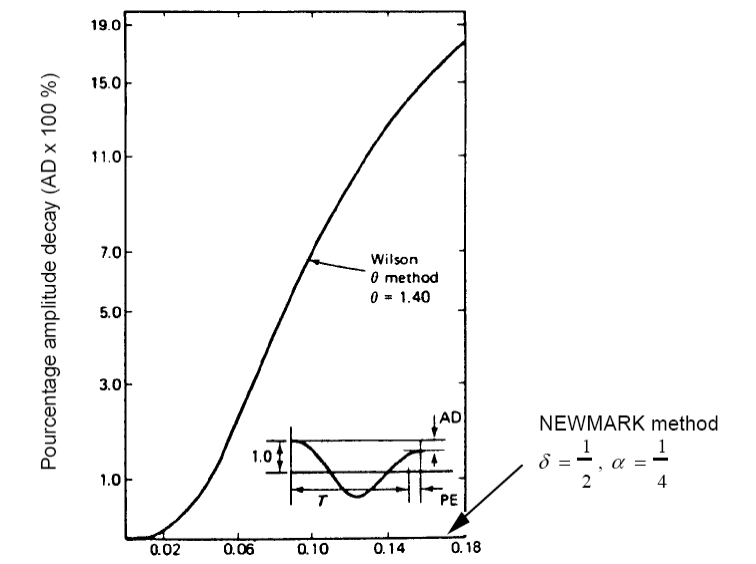
Here we check that the NEwmark algorithm with these parameters does not present any numerical damping.

On the other hand, the implicit algorithms also have a fairly significant effect of extending the natural periods contained in the response of the structure, which leads to a phase shift in the calculated solution. The graph below shows the percentage of elongation of the natural period of a system to a degree of freedom without damping.

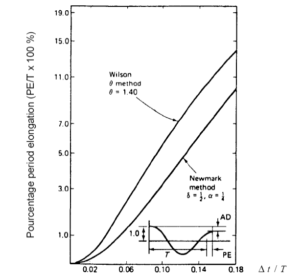
On these two graphs, it can be seen that in order to guarantee precision in the amplitude and the phase of the calculated movements, it is necessary to respect a criterion similar to:

\(\mathrm{\Delta }t<\frac{0.1}{{F}_{\text{max}}}\text{à}\frac{0.01}{{F}_{\text{max}}}\)

where \({F}_{\text{max}}\) is the highest frequency of the movement that we want to capture correctly in numerical analysis.