3. Implementation of the method#

This chapter the implementation of the « LAC » (Local Average Contact) method in*code_aster*. In particular, we will discuss the implementation choices related to the new contact condition by avoiding the creation of new mesh types in code_aster and by integrating into the already existing contact management formalism. It is therefore appropriate for this first version of the implementation of the method to adopt the mesh contact strategy (we will define late contact elements making it possible to carry out the elementary calculations of contact contributions) and a generalized Newton type approach.

The operators impacted by the method are:

CREA_MAILLAGE;
DEFI_CONTACT;
STAT_NON_LINE.

The proposed method involves the following changes:

A modification of the mesh on the slave contact zone (non-invasive in the volume) in operator CREA_MAILLAGE;
A redefinition of contact Lagrangians, implementation of the \({P}^{0}({T}^{M})\) space in the DEFI_CONTACT operator;
A new pairing of the « segment-segment » type in 2D and of the « face-to-face » type in 3D, new evaluation of contact statuses and a new elementary calculation, impact in the operator STAT_NON_LINE and DYNA_NON_LINE.

3.1. Preparing the mesh#

3.1.1. Principles of cutting#

The theoretical basis requires us to satisfy the hypothesis of the degree of internal freedom (see § 2.3). For the sake of simplicity, coherence between 2D and 3D, and in order not to « de-refine » the contact condition, the local refinement method will be used in 2D and 3D cases. The operator’s keyword factor DECOUPE_LAC makes it possible to prepare this macro-mesh. In some situations, the keyword will cut through the cracks, in others, it will not be necessary. When we cut a surface element we therefore make sure not to propagate this cut in the volume. This strategy makes it possible to limit the creation of too many meshes but can cause poor quality meshes.

Likewise, in order to not modify the user’s initial choices, we will always propose a conformable division: a triangle will be cut into triangles, a hexahedron into hexahedra, etc.

3.1.2. The 2D case#

In the 2D case, the slave contact interface is « 1D ». The latter is meshed either in SEG2 or in SEG3. First of all, we note that the SEG3 associated with itself (macro-mesh) satisfies the hypothesis of the internal DDL, so it will not be necessary to cut the meshes that have SEG3 in skin (TRIA6, QUAD8 and QUAD9). In case SEG2, there are two cuts according to the type of associated body mesh. In case TRIA3, we add a knot in the center of the SEG2 mesh and we rebuild the two new skin elements and the two new body elements. In case QUAD4. Since we want to proceed with a consistent cut, we add two knots in mesh SEG2, and two knots in mesh QUAD4. It is then possible to reconstruct the three new skin elements and the four new body elements while providing the information characterizing the macro-mesh. The results of these operations are presented in the table below (the contact surface is shown in blue).

Note: Special attention will be paid to the orientation of the new cells created, to the conformity of the created calculation mesh and to the updating of the mesh groups. Knowing that you cannot update node groups. Indeed, it is not possible to determine whether a new node fits into a group of nodes already defined or not.




TRIA3	TRIA3après DECOUPE_LAC



TRIA6	TRIA6après DECOUPE_LAC (no change)





QUAD4	QUAD4après DECOUPE_LAC



QUAD8	QUAD8après DECOUPE_LAC (no change)





QUAD9	QUAD9après DECOUPE_LAC (no change)

3.1.3. The 3D case#

In the 3D case, the slave contact interface is 2D. The latter can be meshed in TRIA3, TRIA6,, QUAD4, QUAD8, and QUAD9. As in the 2D case, the QUAD9 mesh associated with itself satisfies the internal DDL hypothesis, it is therefore possible to directly fill in the data structures containing the information relating to the macro-mesh without refining locally. In the other cases, two standard cuts will be used, one for the tetrahedral cases, and the other for the hexahedral cases. These two cuts are consistent in the sense that an element is cut by generating the same type of elements. The results of these operations are shown in the table below.




TETRA4	TETRA4après DECOUPE_LAC



	HEXA8après DECOUPE_LAC (Versione 1)



HEXA8	HEXA8après DECOUPE_LAC (Version 2)
HEXA20	Two versions (same as HEXA8)
HEXA27	HEXA27après DECOUPE_LAC (no change)

3.1.4. A few remarks on cutting#

Operator functionality DECOUPE_LAC is capable of processing:

different types of mesh within the same contact zone;
the multi-contact zone.

Regarding the complexity of the calculations on the new mesh, we note that we are adding a certain number of nodes that will carry DDLs and potentially contact Lagrangians. Let M be the number of meshes of the slave surface of the contact zone in question, then for meshes (of bodies) in:

TRIA3 we add \(M\) knots and \(2M\) stitches,
QUAD4 we add \(4M\) knots and \(5M\) stitches,
TETRA4 we add \(M\) knots and \(4M\) stitches,
TETRA10 we add \(5M\) knots and \(4M\) stitches,
HEXA8 (version 1) we add \(8M\) knots and \(9M\) stitches,
HEXA20 (version 1) \(28M\) knots and \(9M\) stitches are added.

In addition, the aspect ratio and the configuration of the meshes generated may possibly interfere with the post-processing of certain data on the slave surface (skin elements and body elements in contact).

3.2. Contact preparation#

The preparation of the contact data is ensured by the operator DEFI_CONTACT. This operator must take into account the new definition of contact Lagrangians, i.e. space \({P}^{0}({T}^{M})\). For each macro-mesh of surface LAC, a contact Lagrangian must be added (see figure) knowing that it is not possible for code_aster to assign a degree of freedom to a physical entity other than a node. We will present here a trick for defining the \({P}^{0}({T}^{M})\) space locally on each computing mesh provided that there is an intelligent assembly of the matrix system.

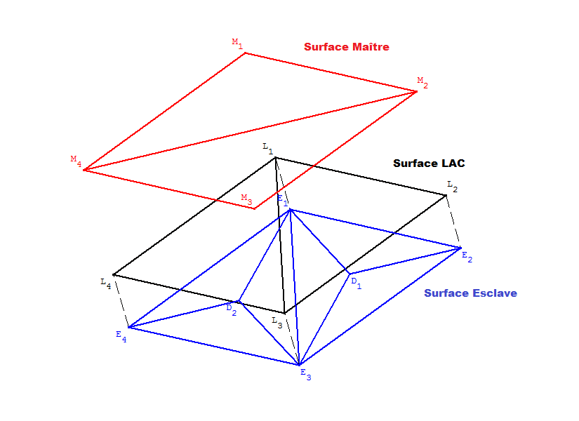
Figure 2: The three spaces in the contact zone (master, slave, and LAC)

3.2.1. Illustration of the technique on case TRIA3#

The trick lies in the fact that we know for each mesh in the slave contact zone of the mesh given by DECOUPE_LAC what is the local number (in connectivity) of the internal node of the macro-mesh, see figure.

Figure 3: Local numbering of the calculation mesh, case TRIA3 (obtained by DECOUPE_LAC)

We therefore know on which node we must add the degree of freedom \(\mathit{LAGS}\text{\_}C\) (see figure), the local number of the node carrying the degree of freedom \(\mathit{LAGS}\text{\_}C\) being fixed we can define only one new type of element making it possible to take into account the location of \(\mathit{LAGS}\text{\_}C\).

Figure 4: Allocation of degrees of freedom on each new slave contact mesh TRIA3

Each degree of freedom \(\mathit{LAGS}\text{\_}C\) is in fact common to only three elements, the three elements making up the macro-mesh. Given that the basic function \({P}^{0}\) associated with the contact Lagrange multiplier does not depend on the geometric vertices of the macro-mesh, it is possible to split the elementary calculation on the macro-mesh into elementary calculation on each cell composing it. During assembly, the contributions of each underlying cell to the macro-mesh are summed. So by assigning to each degree of freedom \(\mathit{LAGS}\text{\_}C\) a base function that is locally constant on the element, we obtain that the degrees of freedom \(\mathit{LAGS}\text{\_}C\) correspond to the space \({P}^{0}({T}^{M})\).

3.2.2. Illustration of the difficulties in case QUAD4#

The case of a slave contact interface meshed in QUAD4 makes it possible to highlight all the difficulties that this trick can cause:

Different local locations of the node associated with degree of freedom \(\mathit{LAGS}\text{\_}C\);
Multiplication of the \(\mathit{LAGS}\text{\_}C\) degree of freedom, due to the fact that we do not have a \(\mathit{LAGS}\text{\_}C\) degree of freedom common to all the cells underlying the macro-mesh.

The second difficulty comes from the fact of the « compliant » division into six HEXA8, see figure.

Figure 5: Local numbering of the calculation mesh, case QUAD4 (obtained by DECOUPE_LAC)

Since we do not have a \(\mathit{LAGS}\text{\_}C\) degree of freedom common to all the cells underlying the macro-mesh, we must locally create four \(\mathit{LAGS}\text{\_}C\) carried by each degree of freedom added. We then notice the first difficulty. There are two types of meshes underlying the macro-mesh, see figures and:

Four stitches with two degrees of freedom \(\mathit{LAGS}\text{\_}C\);
A stitch with the four degrees of freedom \(\mathit{LAGS}\text{\_}C\).

Figure 6: Allocation of degrees of freedom on the new slave contact meshes QUAD4 (type E5)

Figure 7: Allocation of degrees of freedom on the new slave contact meshes QUAD4 (type E1 E2 E3 E4)

During the assignment of the « late » contact elements to the slave contact cells in DEFI_CONTACT, it is necessary to know whether the mesh is of type E5 or E1, E2, E2, E3, E4. We will therefore loop on the macro-meshes and then on the underlying cells knowing that they are ordered in a known manner when updating the group of cells defining the slave surface of the contact zone in question (for example E1, E2, E2, E3, E3, E4 and E5).

It will be treated in STAT_NON_LINE through the use of intelligent assembly. During assembly, we will have to condense the contributions into a single \(\mathit{LAGS}\text{\_}C\), in order to properly impose the local mean contact condition on each \({T}^{m}\) macro-mesh.

3.2.3. Case TRIA6#

This case is similar to case TRIA3, see figure.

Figure 8: Allocation of degrees of freedom on new slave contact meshes TRIA6

3.2.4. Case QUAD8#

This case is similar to case QUAD4, however one does not assign a \(\mathit{LAGS}\text{\_}C\) degree of freedom to the middle nodes (see figures and).

Figure 9: Allocation of degrees of freedom on the new slave contact meshes QUAD8 (type E5)

Figure 10: Allocation of degrees of freedom on the new slave contact meshes QUAD8 (type E1 E2 E3 E4)

3.2.5. Case SEG2#

We must differentiate this case into two sub-cases, the first for SEG2 from TRIA3 and the second for those from QUAD4. These cases are similar to case QUAD4, in fact, as one must maintain the orientation of the meshes, one cannot freely order the nodes in the connectivity of the mesh resulting from operation DECOUPE_LAC. For SEG2/TRIA3, there are two types of mesh (see figures and),

Figure 11: Local numbering of the calculation mesh, case SEG2/TRIA3 (obtained by DECOUPE_LAC)

Figure 12: Allocation of degrees of freedom on slave contact meshes SEG2/TRIA3 For SEG2/QUAD4, there are three types of mesh (see figures and).

Figure 13: Local numbering of the calculation mesh, case SEG2/QUAD4 (obtained by DECOUPE_LAC)

Figure 14: Allocation of degrees of freedom on slave contact meshes SEG2/QUAD4

3.2.6. Cases SEG3 or QUAD9#

It has already been noted that these two types of mesh correspond directly to macro-meshes (the meshes and the macro-meshes are combined). In this case, we therefore have a single element to assign to the contact meshes SEG3 and QUAD9, see figures and.

Figure 15: Allocation of degrees of freedom on slave contact meshes SEG3

Figure 16: Allocation of degrees of freedom on slave contact meshes QUAD9

3.3. Solving the contact problem#

There are three main impacts:

We must have a « segment-segment » type pairing in 2D and a « face-to-face » type pairing in 3D;
Contact matrices must be calculated;
We must develop an assembly of the intelligent global system (management of the second difficulty related to the trick in DEFI_CONTACT, see § 3.2.2).

The first two points require an efficient and robust mesh intersection tool in the case of straight cells (linear and quadratic) and in the case of curved cells (quadratic).

3.3.1. Algorithm for resolving non-linearities related to contact#

We opt for the use of a generalized Newton algorithm, managing geometric nonlinearity, the active constraint strategy for contact nonlinearity and the nonlinearity of behavior within the same Newton loop. This algorithmic framework is already present in code_aster (see [R5.03.52]). It will therefore be sufficient to replace all the internal bricks of the algorithm to implement the new method. We ask:

\[\]

: label: eq-30

U=left [begin {array} {c} {c} {U} _ {N}\ {U} _ {M}\ {U} _ {E}end {array} {U}end {array}right]

textrm {;}

K=left [begin {array} {ccc} {K} {K} {K} _ {NN} & {K} _ {NE} _ {N} _ {MN} & {K} _ {MM} & {K} _ {MM} & {MM} & {MM} & {K} _ {EM} _ {EE} & {K} _ {EE} _ {MM} & {K} _ {EE}{MM}} & {K} _ {EE}{MM} & {K} _ {EE}{MM} & {K} _ {EE}} _ {MM} & {K} _ {EE}} _ {MM} & {K} _ {EE}} _ {MM} & {K} _ {EE}} _ {MM} & {K} _ {EE}} _ `; :math: `C=left [begin {array} {c} {c} 0\ {C} ^ {M}\ {C} ^ {E}end {array}right]

Taking into account the initial « built-in game » \(\overline{{G}_{0}}\) (see definition in §), the problem is equivalent to:

\[\]

: label: eq-31

{begin {array} {c}left [begin {array} {cc} K& Cend {array}right]timesleft [begin {array} {c} U\ mathrm {Lambda}left [begin {array} {Lambda}}end {array} {cc}} K& Cend {array} {cc} K& Cend {array}right} K& Cend {array}right]timesleft [begin {array} {c}} U\mathrm {Lambda}\ Lambda}\ end {array}}right] =F\ {array}right] =F\ {{text {}}} ^ {t}mathit {CU} 0}}text {in} {mathrm {390}}} ^ {k}} ^ {k}\ mathrm {Lambda} ≤0text {in} {mathrm {492}} ^ {k}\ {k}\ {text {}}\ text {in}\ text {in}\ text {in}\ text {in}\ text {in}\ text {in}\ text {in}\ text {in}\ text {in}\ text {in}\ text {in}\ text {in}\ text {in}\ text {in}\ text {in}\ text {in}\ text {in}{text {in}{text {}}\ text {}end {array}

The following function is introduced:

\[\]

: label: eq-32

A (U,Lambda) =Lambda +mathrm {max} (mathrm {0,}rho (CU-overline {{G} _ {0}}) -Lambda)

We can then show that is equivalent to:

(3.1)#\[ \begin{align}\begin{aligned}\begin{split} \ left [\ begin {array} {cc} K& C\ end {array}\ right]\ times\ left [\ begin {array} {c} U\\ Lambda\ end {array}\ right] =F\end{split}\\ \ textrm {and}\\ A (U,\ Lambda) =0\end{aligned}\end{align} \]

The resolution of contact nonlinearity then comes back to the search for active constraints. The contact is active when the status of the point is active, which will be noted \(S{\Lambda }_{i}=1\). The following global algorithm is obtained:

Initial pairing: calculation of \(\overline{{G}_{0}}\)
Loop on the Lagrange \(i=1.\mathrm{.}\mathit{dim}(\mathrm{\Lambda })\)
- If \(\overline{{{G}_{0}}_{i}}⩽0\) then the point is not in contact, so \({\mathrm{\Lambda }}_{i}^{0}=0\)
- If not, the point is in contact, so \({\mathrm{\Lambda }}_{i}^{0}=1\)
Newton loop \(k=1\)
- As long as {\(S{\mathrm{\Lambda }}^{k}\ne S{\mathrm{\Lambda }}^{k+1},\forall k\) and \({\Vert r\Vert }_{2}⩾\mathit{tole}\) (Newton’s equilibrium residue)
  Calculation of stiffness matrices and elementary second members
  
  Calculation of matrices and elementary second contact members
  
  Loop on the Lagrange \(i=1.\mathrm{.}\mathit{dim}(\mathrm{\Lambda })\)
  
  If \(S{\mathrm{\Lambda }}_{i}^{k}=1\) then \(\left[\begin{array}{ccc}0& {C}_{k}^{E}& 0\\ {\text{}}^{t}{C}_{k}^{E}& 0& {\text{}}^{t}{C}_{k}^{M}\\ 0& {C}_{k}^{M}& 0\end{array}\right]\)
  
  Otherwise \(\left[\begin{array}{ccc}0& 0& 0\\ 0& \mathit{Id}& 0\\ 0& 0& 0\end{array}\right]\)
- Assembly of the overall system and resolution:
  \(\left[\begin{array}{ccc}{J}_{k}^{K}& {C}_{k}& 0\\ {\text{}}^{t}{C}_{k}& 0& 0\\ 0& 0& \mathit{Id}\end{array}\right]\times \left[\begin{array}{c}\mathrm{\Delta }{U}_{k}\\ \mathrm{\Delta }{\mathrm{\Lambda }}_{k}^{a}\\ \mathrm{\Delta }{\mathrm{\Lambda }}_{k}^{\mathit{na}}\end{array}\right]=\left[\begin{array}{c}{r}_{k}\\ \overline{{G}_{k}}\\ -\mathrm{\Delta }{\mathrm{\Lambda }}_{k-1}\end{array}\right]\).
- Unknowns update:
  \({U}_{k+1}={U}_{k}+\mathrm{\Delta }{U}_{k}\) and \({\mathrm{\Lambda }}_{k+1}={\mathrm{\Lambda }}_{k}+\mathrm{\Delta }{\mathrm{\Lambda }}_{k}\)
- Matching on updated geometry calculation of \(\overline{{G}_{k+1}}\)
- Evaluation of the new statuses:
  Loop on the Lagrange \(i=1.\mathrm{.}\mathit{dim}(\mathrm{\Lambda })\)
  
  If \({{\mathrm{\Lambda }}_{k+1}}_{i}+\mathrm{\rho }{{G}_{k+1}}_{i}⩽0\) then the point is in contact, so \(S{\mathrm{\Lambda }}_{i}^{k+1}=1\)
  
  Otherwise, the point is not in contact, so \(S{\mathrm{\Lambda }}_{i}^{k+1}=0\)
- Newton residue calculation \({r}_{k+1}\)

3.3.2. Pairing#

The aim of this phase is to manage the geometric nonlinearity of the problem and that resulting from possible large displacements. For each slave contact mesh, the master cells likely to communicate with the slave mesh are sought. During this operation, it is also necessary to calculate the average « clearance » between the two surfaces for each macro-mesh. To do this, we will use four tools:

A linear complexity research tool using neighborhood information at the edge level;
A tool for projecting two cells on the same reference plane (parametric reference space of the slave cell);
A tool for intersecting flat meshes;
A tool for calculating the average distance between a triangle and a surface (3D case) or between two segments (2D case).

3.3.2.1. Linear complexity search algorithm#

The algorithm PANG for calculating the mortar projection matrix for domain decomposition is adapted to the case of contact. This algorithm is of linear complexity once a pair of initial cells has been found. It uses a restricted search on the master neighboring meshes of the master stitches intersecting a slave mesh. In addition, it uses neighborhood information at the slave cell level to update the list of starting cell pairs.

This algorithm saves a significant amount of time compared to a brute-force pairing (i.e. double master-slave pairing loop). However, it lacks robustness. In fact, in the case of a pairing zone that does not have a single connected component, it is failed. Only one of the pairing zones is then detected and the contact algorithm is therefore put in check. A more robust but more expensive version of the initial algorithm is proposed by combining it with a recursive search for a starting pair of cells by brute force.

3.3.2.2. Projection tool#

This tool is already available in code_aster. In fact, one of the matching tools of the CONTINUE method (see [R5.03.52]) performs the orthogonal projection of a point in real space into the parametric space of a given mesh. We will therefore be able to project any master cell into the parametric space of the slave cell in order to perform the intersection test. Two important points are noted:

We are limited to the case where the projection of the master mesh into the slave parametric space is**convex*;

Since the projection is carried out in the parametric space of the master mesh, we will only achieve a purely \(1D\) or \(2D\) intersection.

In addition, another routine is available in code_aster: projection under an imposed direction. Note that this projection algorithm will be useful for the average « game » tool.

3.3.2.3. Medium « game » tool#

This tool is introduced in the 2D case described in the figure. The slave mesh consists of two cells (\(E1\), \(E2\)) and therefore a macro-mesh associated with a degree of freedom \(\mathit{LAGS}\text{\_}C\); the master mesh also consists of two cells (\(M1\), \(M2\)).

Figure 17:2D configuration studied, in blue the master cells M1 and M2, in red the slave cells E1 and E2

By combining the projection and intersection tools, the contact meshes described in the figure are obtained. The average game tool on the first contact mesh will be described.

Figure 18: Contact meshes obtained by the first two operations of the pairing

If we perform the operations projection on the slave cell and intersection, we obtain the projections of the points \({Y}_{1}\) and \({Y}_{2}\) in the reference space of the slave cell \(E1\), respectively \({P}_{1}\) and \({P}_{2}\), and the intersection (magenta segment). The result of these operations is shown in the figure.

Figure 19: Projection and intersection in the reference space of the slave cell \(E1\)

By considering the intersection as a pseudoelement, we can report the Gauss points resulting from a quadrature formula in the reference space of the slave cell. For simplicity, we consider here a quadrature formula at a Gauss point \(\mathit{Pg}\); its associated weight is the weight of the intersection. We then go back to real space to be able to estimate the distance to the Gauss points. These operations are described in the figure.

Figure 20: Gauss point game, \(d\)

The following contribution is added to the component of the « integrated game » vector, \(\overline{G}\), corresponding to the degree of freedom \(\mathit{LAGS}\text{\_}C\) of the contact mesh:

(3.2)#\[\begin{split} {\ overline {G}} _ {\ mathit {LAGS}\ text {\ mathit {}}\\\ text {\ mathit {}}\ text {\ _} C} +\ sum _ {i=1}\ sum _ {i=1}\ ^ {i=1}\ ^ {N} {1}} ^ {N} {d} _ {d} _ {i}} _ {i}\ Vert ({\ partial} _ {1}\ 1}\ green ({\ partial} _ {1}\)\ mathrm {\ sigma}\ times {\ partial} _ {2}\ mathrm {\ sigma}) ({\ mathit {Pg}} _ {i}) {\ green} _ {i}) {\ green} _ {2} LAGS\end{split}\]

where \({d}_{i}\) is the game signed at the i-th Gauss point (\({\mathit{Pg}}_{i}\)), \({\mathrm{\omega }}_{i}\) is the weight associated with the i-th Gauss point in the reference space of the master cell of the contact mesh, \(\mathrm{\sigma }\) is the transition transformation reference element real element and \(N\) is the number of Gauss points defined on the intersection.

By iterating on the contact cells, we obtain the vector \(\overline{G}\) whose dimension corresponds to the number of degrees of freedom \(\mathit{LAGS}\text{\_}C\); in our example there is no single component in the integrated « game » vector.

In the three-dimensional case, a convex polygon triangulation tool is required. Indeed, it is easier to calculate the \(\overline{G}\) piecewise on a set of triangles (simpler definition of quadrature formulas than on any polygon).

To finish the operation, simply divide each component of the integrated « game » vector by the intersection weight found on the associated macro-mesh.

3.3.2.4. Management of quadratic meshes#

In the curved quadratic case, it is not possible to approach the geometry of the master cell in the slave parametric space. To simplify the algorithm, we will use simple linearization instead of decomposing the mesh into linear elements commonly used in the literature on mortar methods for contact. For its part, slave geometry is approximated exactly by its parametric space. Contrary to the current approach consisting in using an auxiliary intersection plane (defined from the slave surface), it was chosen to perform all the projection and intersection operations in the slave parametric space. This choice allows both the use of a matching tolerance criterion independent of the modeling and to perform only purely \(2D\) or \(1D\) intersections. By using this approach and by controlling the quality of the mesh, we prevent the appearance of severe pathological cases that result in fatal errors or in a non-convergence of the generalized Newton algorithm. Moreover, unlike the classic \(P2/P2\) mortar methods, the LAC method does not face the sign problem with respect to the basic functions of the Lagrange multiplier space. Attention should therefore be paid mainly to the quality of the mesh, and more particularly to the mesh of the slave surface. In fact, the algorithmic choices implemented in this first version of the implementation of the method do not take into account the case of non-convex intersections. If the slave cells do not respect this constraint, irrelevant intersections are obtained. Aberrant intersection coefficients (greater than one) are therefore observed, which results in a failure of convergence of the algorithm for solving the problem.

3.3.3. Calculation of contact matrices#

The calculation of the elementary contact matrices is directed by the status field \(\mathit{S\Lambda }\). If the constraint associated with macro-element \(T\) is active, then the following contributions must be calculated:

(3.3)#\[ \begin{align}\begin{aligned} {C} _ {i} ^ {{M} _ {\ mathit {elem}}}} = {\ int} _ {T} {\ phi} _ {i} ^ {M} {\ vec {n}}} _ {m}} _ {m} d\ d\ d\ Gamma =\ Gamma =\ sum =\ sum _ {M} _ {e}} {e}} {\ phi} _ {i} ^ {M} {\ vec {n}} _ {m} d\ Gamma\\ {C} _ {i} ^ {{E} _ {\ mathit {elem}}}} = {\ int} _ {T} {\ phi} _ {i} ^ {E} {\ vec {n}}} _ {e}} _ {e} d\ d\ d\ Gamma =\ sum =\ sum _ {M} _ {e}} {e}} {e}} {\ phi} _ {i} ^ {E} {\ ve} {\ vec {n}} _ {e} d\ Gamma\end{aligned}\end{align} \]

where \({\phi }^{E}\) and \({\phi }^{M}\) are the slave and master database functions, \({\vec{n}}_{e}\) and \({\vec{n}}_{m}\) the respective normals, \({M}_{c}\) the set of contact cells, and \({M}_{E}\) the set of slave cells. If the contact stress associated with the macro-element \(T\) is inactive then there are no contact conditions to be respected on this macro-element and the associated degree of freedom \(\mathit{LAGS}\text{\_}C\) is set to zero. Since the macro-mesh \(T\) does not exist as an element, « sub-elementary » matrices will be calculated at the level of contact cells \({M}_{c}\) (association of a slave and master contact mesh).

3.3.3.1. Calculation of elementary contact matrices#

In fact, we calculate the elementary contact matrices \({C}^{{M}_{\mathit{elem}}}\) corresponding to the integrals under the loop on the contact cells (see equations). For each contact mesh, the following matrices must be calculated:

(3.4)#\[ \begin{align}\begin{aligned} {C} _ {i} ^ {{M} _ {\ mathit {elem}}}} = {\ int} _ {{M} _ {m}\ cap {M} _ {e}} {\ phi}} {\ phi} _ {\ phi} _ {i} _ {m}\ mathit {d\ Gamma} _ {m}\ mathit {d\ Gamma}} {\ phi}} _ {e}} {\ phi} _ {e}} {\ phi} _ {e}} {\ phi} _ {e}} {\ phi} _ {e}} {\ phi} _ {e}} {\ phi} _ {e}}\\ {C} _ {i} ^ {{E} _ {\ mathit {elem}}}} = {\ int} _ {{M} _ {m}\ cap {M} _ {e}} {\ phi}} {\ phi} _ {\ phi} _ {e}} {\ phi}} _ {e}} {\ phi}}} {\ phi} _ {e}} {\ phi}} _ {e}} {\ phi}} _ {e}} {\ phi}} _ {e}} {\ phi}} _ {e}} {\ phi}} _ {e}} {\ phi}} _ {e}} {\ phi}}\end{aligned}\end{align} \]

where \({M}_{e}\) is the contact mesh slave and \({M}_{m}\) is the contact mesh master. Since the contact condition chosen corresponds to a zero game only on average, a projection-intersection must be carried out to define the integration medium. To do this, we reuse the tools presented in the previous section. By following the diagram of the integrated game tool, we manage to obtain the coordinates and weights of a quadrature formula in the parametric space of the slave cell of the contact mesh. By looping over the degrees of freedom of master movements, we can then calculate the coefficients of the matrix \({C}_{i}^{{E}_{\mathit{elem}}}\). Then, using the projection onto the parametric space of the master cell of the contact mesh, we then obtain the integration support in the reference space of the master cell, which makes it possible to calculate (by defining an integration diagram) the coefficients of the matrix \({C}_{i}^{{M}_{\mathit{elem}}}\).

3.3.3.2. Choosing the normal#

The question of choosing the normal one has not yet been addressed. As this choice is not a unique step, we propose to use two types of normal in our case. Either we evaluate the normal at each master and slave Gauss point, or we use a field of smoothed normals (keyword LISSAGE =” OUI “) calculated on each deformed configuration (master and slave). These two choices make it possible to avoid the problem of multiple definition of the normal at the top of the elements when considering curved geometries. In the quadratic case, these two choices are relatively similar; on the contrary, in the case of linear meshes, the smoothed normal field makes it possible to regularize the normal field and to better approach the curved geometries, see figure.

Figure 21: Different choices of normal fields

3.3.4. Smart assembly#

Here we present a way to manage the second difficulty related to the trick used in DEFI_CONTACT. We are in case HEXA8; we want to calculate the matrix \({C}^{E}\). It is assumed that the slave mesh is only composed of a macro-mesh, so there are five cells on the slave surface (for simplicity we will only talk about slave contributions), eight degrees of freedom of movement, four « computer » contact Lagrangians, but only one Lagrangian in the mathematical sense. The figure shows the slave mesh in question.

Figure 22: Slave mesh, in black (\({x}_{1}\),…,…, 4) the degrees of freedom of movement, in red (1,…, 4) the « computer » Lagrange degrees of freedom. \({x}_{4}\) \({d}_{1}\) \({d}_{4}\)

The elementary matrices are as follows:

Item I:

(3.5)#\[\begin{split} \ left [\ begin {array} {cccc} {a} {a} _ {I} & {b} _ {I} & {c} _ {I} & {d} _ {I}\ {a} _ {I} & {b} & {b} _ {I} & {b} _ {I} & {c} _ {I} & {d} _ {I}\ end {array}\ right]\ times\ {a} _ {I} _ {I}} _ {I}\ {a} _ {I}} _ {I}\ {a} _ {I}} _ {I}\ {a} _ {I}} _ {I}\ {a} _ {I}} _ {I}\ {a} _ {I}} _ {I}\ {a} _ {I}} c} {x} _ {1}\\ {x} _ {2}\\ {x} _ {2}\\ {d} _ {1}\ end {array}\ right] =\ left [\ begin {array} {c}\ textcolor [array} {c} {c}\ textcolor [rgb] {1,0,0} {2}\ end {array} {c} {c}\ textcolor [rgb] {1,0,0} {2}\ end {array} {c} {c}\ textcolor [rgb] {1,0,0} {2}\ end {array} {c} {c}\ textcolor [rgb] {1,0,0} {2}\ end {array} {c} {c}\ textcolor [rgb] {1,0,0} {2}\ end {array} {c}\end{split}\]

Element II:

(3.6)#\[\begin{split} \ left [\ begin {array} {cccc} {a} _ {\ mathit {II}} _ {\ mathit {II}}} & {\ mathit {II}} & {\ mathit {II}}} & {d}} _ {\ mathit {II}} _ {\ mathit {II}}} & {c}} _ {\ mathit {II}}} & {c} _ {\ mathit {II}}} & {c} _ {\ mathit {II}} & {d} _ {\ mathit {II}}}\ end {array}\ right]\ times\ left [\ begin {array} {c} {x} _ {2}\\ {x} _ {2}\\ {x} _ {3}\\ {x} _ {3}\\ {d} _ {2}\ end {array}\ right] _ {2}\\ {array}\ right] =\ left [\ begin {x}} _ {2}\\ {array}\ right] =\ left [\ {x}} _ {2}\\ {x} _ {2}\\ {x} _ {2}\\ {x} _ {2}\\ {x} _ {2}\\ {x} _ {2}\\ {array}}\ textcolor [rgb] {1,0,0} {2} {2}\\\ textcolor [rgb] {1,0,0} {3}\ end {array}\ right]\end{split}\]

Item III:

(3.7)#\[\begin{split} \ left [\ begin {array} {cccc} {a} _ {\ mathit {III}} _ {\ mathit {}}} & {\ mathit {III}} & {\ mathit {III}}} & {d}} & {d} _ {\ mathit {III}} _ {\ mathit {}}} _ {\ mathit {}}} _ {\ mathit {}}} _ {\ mathit {}}} _ {\ mathit {}}} _ {\ mathit {}}} _ {\ mathit {}}} _ {\ mathit {}}} _ {\ mathit {}}} _ {\ mathit {}}} _ {\ mathit {}}} _ {\ mathit {}}} {\ mathit {III}} & {d} _ {\ mathit {II}} {\ mathit {II}}}\ end {array}\ right] I\ times\ left [\ begin {array} {x} _ {3}\\ {x} _ {3}\\ {x} _ {3}\\ {array} {x} _ {3}\ end {array} {x} _ {3}\\ {array} {x} _ {3}\\ {x} _ {3}\\ {x} _ {3}\\ {x} _ {3}\\ {x} _ {3}\\ {x} _ {3}\\ {x} _ {3}\\ {x} _ {3}\\ {x} _ {3}\\ {x} _ {3} c}\ textcolor [rgb] {III III 1,0,0} {3}\\\ textcolor [rgb] {1,0,0} {4}\ end {array}\ right]\end{split}\]

Element IV:

(3.8)#\[\begin{split} \ left [\ begin {array} {cccc} {a} _ {\ mathit {IV}} _ {\ mathit {IV}}} & {\ mathit {IV}} & {\ mathit {IV}}} & {d}} _ {\ mathit {IV}} _ {\ mathit {IV}}} & {c}} _ {\ mathit {IV}}} & {c} _ {\ mathit {IV}}} & {c} _ {\ mathit {IV}} & {d} _ {\ mathit {IV}} {\ mathit {IV}}}\ end {array}\ right]\ times\ left [\ begin {array} {x} _ {4}\\ {x} _ {4}\\ {x} _ {4}\\ {array} _ {4}\ end {array}\\} _ {4}\ end {array}\\} _ {4}\\ {x} _ {4}\\ {x} _ {4}\\ {x} _ {4}\\ {x} _ {4}\\ {x} _ {4}\\ {x} _ {4}\\ {x} _ {4}\\ {x} _ {4}\\ {x} _ {4}\\ {x}\ textcolor [rgb] {1,0,0} {4} {4}\\\ textcolor [rgb] {1,0,0} {1}\ end {array}\ right]\end{split}\]

Element V:

(3.9)#\[\begin{split} \ left [\ begin {array} {cccc} {a} {a} _ {V} & {b} _ {V} & {c} _ {V} & {d} _ {V}\ {a} _ {V} & {b} & {b} & {b} _ {V} & {b} _ {V} & {b} & {b} & {b} & {b} _ {V} & {b} & {b} _ {V} & {b} & {b} _ {V} & {b} & {b} & {b} _ {V} & {b} & {b} _ {V} & {b} & {b} _ {V} & {b} & {b} _ {V} & {b} & {b} _ {V} & {b} & c} _ {V} & {d} _ {V}\\ {a} _ {V} _ {V} & {b} _ {V} & {d} _ {V}\ end {array}\ right]\ end {array}\ right]\ times\ left]\ times\ left [\ times\ left [\ times\ left] [\ {left] [\ left] [\] left [\ begin {array} {a} _ {1}\\ left [\ begin {array} {a}\ left [\ begin {array} {a}\ left [\ begin {array} {a}\ left [\ begin {array} {a}\ left [\ begin {array} {a}\ left [\ begin {array} {a}\ left [\ begin {array} {a}\ left [\ begin {array} {d} _ {4}\ end {array}\\ right] =\ left [\ begin {array} {c}\ textcolor [rgb] {1,0,0} {1}\\ textcolor [rgb] {1,0,0} {2} {2}\\\ textcolor [rgb] {1,0,0} {2}\\ textcolor [rgb] {1,0,0} {4}\ end {array} {2} {2}\\\ textcolor [rgb] {1,0,0} {2}\ end {array} {2}\\ textcolor [rgb] {1,0,0} {2}\ end {array} {2}\\ textcolor [rgb] {1,0,0} {2}\ end {array}\ {right]\end{split}\]

A classical assembly would give us the following global matrix \({C}^{E}\):

(3.10)#\[\begin{split} \ left [\ begin {array} {cccccccc} {a} _ {I}} _ {I} + {b} _ {\ mathit {IV}}} & {b} _ {a} _ {\ mathit {IV}} _ {IV}}} & {a} {IV}}} & {\ mathit {IV}} _ {IV}} _ {V}} & {b} _ {V}} & {b} _ {V}} + {d} _ {I} & {c} _ {V} & {d} _ {V} & {d} _ {V} + {d} _ {IV}}\\ {a} _ {I} & {a} _ {\ mathit {II}} _ {II}}} + {\ mathit {II}}} & {a} _ {V} _ {V}}} _ {V}}} + {c} _ {I} & {b} _ {V} + {d} _ {I} _ {I} + {I} + {I} + {d} _ {V} + {c} _ {\ mathit {II}}} & {d}} & {d} _ {V} _ {V}\\ V}\\ V}\\ 0& {a} _ {a} _ {\ mathit {III}} & {b} _ {\ mathit {III}}} & {a} _ {V} & {b} _ {V} + {d} _ {\ mathit {II}}} & {c}} _ {V} _ {V} + {v}} + {\ mathit {II}} _ {\ mathit {II}}} + {d} _ {\ mathit {II}}} & {\ mathit {II}}} & {\ mathit {II}}} & {\ mathit {II}}} & {\ mathit {II}}} & {\ mathit {II}}} & {\ mathit {II}} III}} & {d} _ {V} + {c} _ {\ mathit {III}} {\ mathit {}}}\\ {b} _ {\ mathit {IV}}} & {\ mathit {III}}} & {\ mathit {}}} & {\ mathit {}}} & {\ mathit {IV}} _ {V}} & {\ mathit {}}} _ {v}} & {\ mathit {}}}} & {\ mathit {}}} & {\ mathit {}}}} & {\ mathit {}}} & {\ mathit {}}}} & {\ mathit {}}} & {\ mathit {}}}} & {\ mathit {}}} it {IV}} & {b} _ {V} & {V} & {c} & {c} & {c} & {c} _ {V} + {c} _ {\ mathit {III}} + {\ mathit {}}} + {\ mathit {}}} + {\ mathit {}}}\ end {array}\ right] III III\end{split}\]

It is easy to notice that this matrix does not correspond to the coupling of movements with functions \({P}^{0}({T}^{M})\). We must find an assembly technique compatible with the assembly used in code_aster (and which should not be totally incompatible with parallelism) making it possible to obtain the following coupling matrix:

(3.11)#\[\begin{split} {\ text {}} ^ {t}\ mathit {DEPL}\ times\ left [\ begin {array} {c} {a} _ {I} + {b} _ {\ mathit {IV}}\\ {b}}\\ {b}} _ {I} _ {I}} _ {I} + {I}} _ {\ mathit {II}}} + {\ mathit {II}}} + {a} _ {\ mathit {II}}} + {a} _ {\ mathit {II}}} + {a} _ {\ mathit {II}}} + {a} _ {\ mathit {II}} III}}\\ {b} _ {\ mathit {III}}} + {\ mathit {}} + {\ mathit {IV}} + {c} _ {I} + {c} _ {c} _ {c} _ {\ mathit {IV}} _ {IV}}}} + {a} _ {V}} + {d} _ {I} _ {c} _ {V} _ {V} + {d} _ {\ mathit {III}} + {c}} _ {\ mathit {II}}\\ {d} _ {V} + {c} _ {\ mathit {III}}} + {d}} + {d} _ {\ d} _ {\ mathit {IV}}}\ end {array}\ right] = {\ mathit { LAG}} _ {C}\end{split}\]

During the elementary assembly, we therefore want to multiply the contributions by \(\frac{1}{2}\) in the case of elements of type E1, E2, E3 and E4 (elementary matrices (), (), () and ()) and by \(\frac{1}{4}\) in the case of elements of type E5 (elementary matrix ()). Then, for each macro-element, the corresponding rows of the global matrix of the system are summed up and only one Lagrangian is kept in the system corresponding to the mathematical contact condition. The three additional computer Lagrangians are set equal to the physical Lagrange multiplier.

3.3.5. Post-treatment#

All contact resolution variables, statuses, Lagrange multipliers, « game », are only relevant at the macro-mesh level, the output field is named CONT_ELEM.