2. Implementation in Code_Aster#

The FONDA_SUPERFI behavior relationship is assigned to discrete modeling elements DIS_TR in 1 node. This relationship is called by the nonlinear problem solving operators STAT_NON_LINE [R5.03.01] or DYNA_NON_LINE [R5.05.05].

The local axes of these x, y, z elements are defined as on the.

Integrating this relationship of assembly behavior into the operator STAT_NON_LINE of Code_Aster requires the formulation of the \(\Delta F\) force increment and the tangent operators \({K}_{o}^{tan}\) and \({K}_{n}^{tan}\).

\(\Delta F\) is the loading increment during the time step (i.e. between \(>\) and \(>\)) caused by a movement increment \(\Delta U\) at this same time step.
\({K}_{n}^{tan}\) is the tangent stiffness at the end of the time step, instant \(>\).
\({K}_{o}^{tan}\) is the tangent stiffness at the start of the time step, instant \(t\) equal to the tangent stiffness at the end of the previous step.

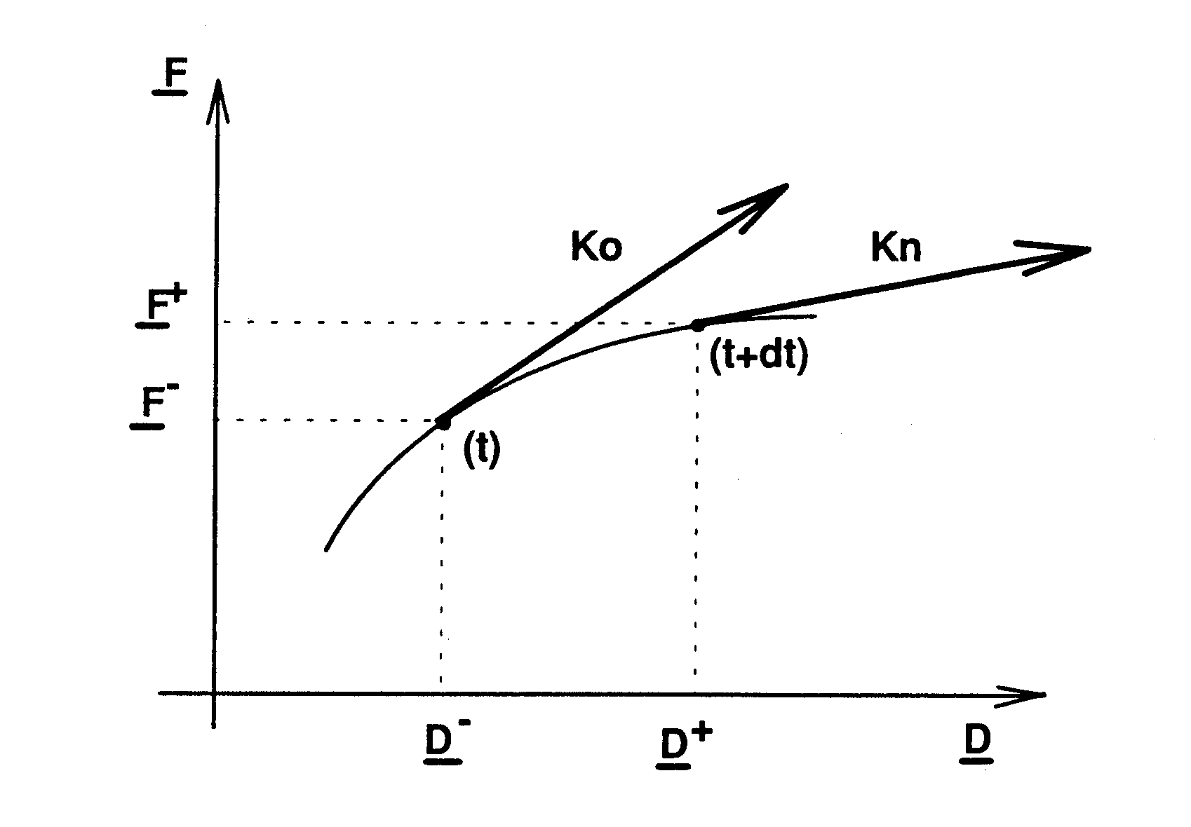
Figure 2-1: Definition of operators \({K}_{o}^{tan}\) and \({K}_{n}^{tan}\)

2.1. Determining the load increment#

2.1.1. Input data#

In addition to the parameters of the law of behavior, variables at the start of the time step (O) are available as input:

global strength: \({F}^{O}={}^{T}\left({F}_{x}^{o},{F}_{y}^{o},{F}_{z}^{o},{M}_{x}^{o},{M}_{y}^{o},{M}_{z}^{o}\right)\text{ }\);
of displacement: \({U}^{O}={}^{T}({u}_{x}^{o},{u}_{y}^{o},{u}_{z}^{o},{\theta }_{x}^{o},{\theta }_{y}^{o},{\theta }_{z}^{o})\text{ }\);
internal variables for sliding work hardening: \({Q}_{sl}^{o}={}^{T}({q}_{{h}_{x}}^{O},{q}_{{h}_{y}}^{O})\text{ }\);
sliding plastic displacement: \({U}_{sl}^{O}={}^{T}({u}_{x,s}^{pl,O},{u}_{y,s}^{pl,O},{u}_{z,s}^{pl,O},{\theta }_{x,s}^{pl,O},{\theta }_{y,s}^{pl,O})\text{ }\);
work-hardening variables in load bearing capacity: \({Q}_{sl}^{o}={}^{T}({R}_{h,x}^{O}\text{ },{R}_{h,y}^{O},{R}^{O},{R}_{m,x}^{O},{R}_{m,y}^{O})\text{ }\);
plastic displacement in CP: \({U}_{\mathit{CP}}^{O}={}^{T}({u}_{x,\mathit{CP}}^{pl,O},{u}_{y,\mathit{CP}}^{pl,O},{u}_{z,\mathit{CP}}^{pl,O},{\theta }_{x,\mathit{CP}}^{pl,O},{\theta }_{y,\mathit{CP}}^{pl,O})\text{ }\);
intermediate internal variables in sliding and CP: \({v}_{x,s}^{pl,O}\), \({v}_{y,s}^{pl,O}\) and \({v}_{z,CP}^{pl,O}\);

As well as the final move at the end of the time step: \({U}^{F}={}^{T}({u}_{x}^{F},{u}_{y}^{F},{u}_{z}^{F},{\theta }_{x}^{F},{\theta }_{y}^{F},{\theta }_{z}^{F})\)

You need all the variables at the end of the time step (notation « F » instead of « O »)

2.1.2. Composition of the tangent elastic matrix#

An initial stiffness matrix \({K}^{ini}\) must be assigned to the discrete element. This matrix must be symmetric and diagonal in its local coordinate system (non-diagonal terms are ignored).

The first step consists in starting from the global force \({F}^{O}\) at the beginning of the time step to calculate the tangent elastic stiffness in rotation according to x \({K}_{\mathit{rx},\mathit{rx}}^{tan,o}\) and y \({K}_{\mathit{ry},\mathit{ry}}^{tan,o}\) with the formulation seen in [§ 1.4] so we obtain the tangent elastic stiffness matrix:

\({K}_{élas}^{o,tan}=\left(\begin{array}{cccccc}{K}_{\mathit{xx}}^{ini}& 0& 0& 0& 0& 0\\ 0& {K}_{\mathit{yy}}^{ini}& 0& 0& 0& 0\\ 0& 0& {K}_{\mathit{zz}}^{ini}& 0& 0& 0\\ 0& 0& 0& {K}_{\mathit{rx},\mathit{rx}}^{tan,o}& 0& 0\\ 0& 0& 0& 0& {K}_{\mathit{ry},\mathit{ry}}^{tan,o}& 0\\ 0& 0& 0& 0& 0& {K}_{\mathit{rz},\mathit{rz}}^{ini}\end{array}\right)\)

2.1.3. Bungee shooting#

From the tangent elastic stiffness matrix, we calculate the force

\({F}^{élas}={}^{T}\left({F}_{x}^{élas},{F}_{y}^{élas},{F}_{z}^{élas},{M}_{x}^{élas},{M}_{y}^{élas},{M}_{z}^{élas}\right)\) that would be obtained if no plasticity mechanism is used (also called « elastic shooting »). Either:

\({F}^{élas}={F}^{O}+{K}_{élas}^{O,tan}\cdot \left({U}^{F}-{U}^{O}\right)\)

2.1.4. Calculation of plastic flow#

Now we calculate \({f}_{\mathit{CP}}\left({F}^{élas},{Q}_{\mathit{CP}}^{O}\right)\) and \({f}_{s}\left({F}^{élas},{Q}_{sl}^{O}\right)\), see § 1.3 and § 1.2.

2.1.4.1. If \({f}_{\mathit{CP}}\le 0\) and \(>\)#

So no plasticity mechanism is achieved, the foundation is in the elastic domain, the elastic pull corresponds to the force at the end of the time step: \({F}^{F}={F}^{élas}\) and no plasticity variable changes:

\({Q}_{sl}^{F}={Q}_{sl}^{O}\text{ },{U}_{sl}^{F}={U}_{sl}^{O},{v}_{x,s}^{pl,F}={v}_{x,s}^{pl,O},{v}_{y,s}^{pl,F}={v}_{y,s}^{pl,O},\text{ }{Q}_{\mathit{CP}}^{F}={Q}_{\mathit{CP}}^{O}\text{ },{U}_{\mathit{CP}}^{F}={U}_{\mathit{CP}}^{O}\text{ }et\text{ }{v}_{z,\mathit{CP}}^{pl,F}={v}_{z,\mathit{CP}}^{pl,O}\)

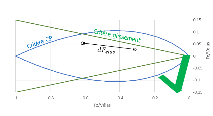
Figure 2.1-1: Illustration of elastic shooting without reaching a breaking mechanism

2.1.4.2. If \({f}_{\mathit{CP}}>0\) and \(>\)#

Only the mechanism of loss of load-bearing capacity is achieved, no plasticity variable related to sliding changes:

\({Q}_{sl}^{F}={Q}_{sl}^{O}\text{ },{U}_{sl}^{F}={U}_{sl}^{O},{v}_{x,s}^{pl,F}={v}_{x,s}^{pl,O},{v}_{y,s}^{pl,F}={v}_{y,s}^{pl,O}\)

We then look for the correction during loading \({dF}^{cor}\text{ }\) and the evolution of the work-hardening variables \({\mathrm{d}Q}_{\mathit{CP}}\) necessary to return to the criterion, namely:

\({f}_{\mathit{CP}}({F}^{élas}-{\mathrm{d}F}^{cor},{Q}_{\mathit{CP}}^{O}+\mathrm{d}{Q}_{\mathit{CP}})=0\)

This equation is solved by an iterative loop until convergence, by writing in iteration k the limited expansion of this equation around point \(({F}^{ité,k},{Q}_{\mathit{CP}}^{ité,k})\):

\({f}_{\mathit{CP}}\left({F}^{élas}-{\mathrm{d}F}^{cor},{Q}_{\mathit{CP}}^{O}+\mathrm{d}{Q}_{\mathit{CP}}\right)\approx \left\{\begin{array}{c}{f}_{\mathit{CP}}\left({F}^{ité,k},{Q}_{\mathit{CP}}^{ité,k}\right)\\ +{}^{T}\left(\frac{\partial {f}_{\mathit{CP}}}{\partial F}\left({F}^{ité,k},{Q}_{\mathit{CP}}^{ité,k}\right)\right)\left({F}^{élas}-{\mathrm{d}F}^{cor}-{F}^{ité,k}\right)\\ +{}^{T}\left(\frac{\partial {f}_{\mathit{CP}}}{\partial {Q}_{\mathit{CP}}}\left({F}^{ité,k},{Q}_{\mathit{CP}}^{ité,k}\right)\right)\left({Q}_{\mathit{CP}}^{O}+{\mathrm{d}Q}_{\mathit{CP}}-{Q}_{\mathit{CP}}^{ité,k}\right)\end{array}\right\}=0\)

Starting with the iterative loop: \(({F}^{ité,0},{Q}_{\mathit{CP}}^{ité,0})=({F}^{élas},{Q}_{\mathit{CP}}^{O})\)

The correction in loading and the evolution of work hardening can be linked to the plastic displacement increment \({\mathrm{d}U}_{\mathit{CP}}^{k}\) by the following relationships:

\({\mathrm{d}F}^{cor}={K}_{élas}^{O,tan}\cdot {\mathrm{d}U}_{\mathit{CP}}^{k}\) and \({\mathrm{d}Q}_{\mathit{CP}}={I}_{CP}^{O}\cdot {\mathrm{d}U}_{\mathit{CP}}^{k}\)

Where \({I}_{\mathit{CP}}^{O}\text{ }\) is calculated with the parameters at the start of the time step (see § 1.3).

We assume that the plastic flow is normal to the plasticity surface, so we relate the plastic increment to the plastic flow variable \(\mathrm{d}{\lambda }_{\mathit{CP}}^{k}\):

\({\mathrm{d}U}_{CP}^{k}=\frac{\partial {f}_{\mathit{CP}}}{\partial F}\left({F}^{ité,k},{Q}_{\mathit{CP}}^{ité,k}\right)\mathrm{d}{\lambda }_{\mathit{CP}}^{k}\)

Thus we can write to obtain an approximation of the plastic flow:

\(\mathrm{d}{\lambda }_{\mathit{CP}}^{k}=\frac{{f}_{\mathit{CP}}\left({F}^{ité,k},{Q}_{\mathit{CP}}^{ité,k}\right)+{}^{T}\left(\frac{\partial {f}_{\mathit{CP}}}{\partial F}\left({F}^{ité,k},{Q}_{\mathit{CP}}^{ité,k}\right)\right)\left({F}^{élas}-{F}^{ité,k}\right)+{}^{T}\left(\frac{\partial {f}_{\mathit{CP}}}{\partial {Q}_{\mathit{CP}}}\left({F}^{ité,k},{Q}_{\mathit{CP}}^{ité,k}\right)\right)\left({Q}_{\mathit{CP}}^{O}-{Q}_{\mathit{CP}}^{ité,k}\right)}{\left({}^{T}\left(\frac{\partial {f}_{\mathit{CP}}}{\partial F}\left({F}^{ité,k},{Q}_{\mathit{CP}}^{ité,k}\right)\right){K}_{élas}^{O,tan}-{}^{T}\left(\frac{\partial {f}_{\mathit{CP}}}{\partial {Q}_{\mathit{CP}}}\left({F}^{ité,k},{Q}_{\mathit{CP}}^{ité,k}\right)\right){I}_{\mathit{CP}}^{O}\right)\times \left(\frac{\partial {f}_{\mathit{CP}}}{\partial F}\left({F}^{ité,k},{Q}_{\mathit{CP}}^{ité,k}\right)\right)}\)

From the plastic flow \(\mathrm{d}{\lambda }_{\mathit{CP}}^{k}\), \({\mathrm{d}U}_{\mathit{CP}}^{k}\), \({\mathrm{d}F}^{cor}\) and \({\mathrm{d}Q}_{\mathit{CP}}\) are deduced, and the failure criterion is reevaluated:

si:math: left| {f} _ {mathit {CP}}}left ({F} ^ {elas} - {mathrm {d} F} ^ {cor}, {Q} _ {Q} _ {mathit {CP} _ {mathit {CP}} _ {mathit {CP}}}right)Q} _ {mathit {CP}} _ {mathit {CP}} _ {mathit {CP}} _ {mathit {CP}} _ {mathit {CP}} _ {mathit {CP}} _ {mathit {CP}} _ {mathit {CP}} _ {mathit {CP}} _ {mathit {CP}} _ {mathit {CP}} _ {mathrm {error} then we have reached the convergence of the correction;
otherwise we start the loop again with:

\(\left({F}^{ité,k+1},{Q}_{\mathit{CP}}^{ité,k+1}\right)=\left({F}^{élas}-{\mathrm{d}F}^{cor},{Q}_{\mathit{CP}}^{O}+{\mathrm{d}Q}_{\mathit{CP}}\right)\)

After convergence of the loop at iteration « m », the plasticity parameters related to the bearing capacity are updated:

math:: {Q} _ {mathit {CP}}} ^ {CP}} ^ {F} = {Q} _ {mathit {CP}}} ^ {U} _ {mathit {CP}}} ^ {F}} ^ {F} = {F} = {U} = {U} _ {U} _ {mathit {CP}}} ^ {O} + {mathrm {d} U} _ {mathit {CP}}} ^ {m}, {v} _ {z,mathit {CP}}} ^ {pl, F}} = {v} _ {z,mathit {CP}} ^ {pl, O} +left|left|mathrm {d} {d} {d} {U}} _ {z,mathit {CP}}} ^ {pl, m+1}right|

We also recover the strength at the end of the time step:

\({F}^{F}={F}^{ité,m+1}\)

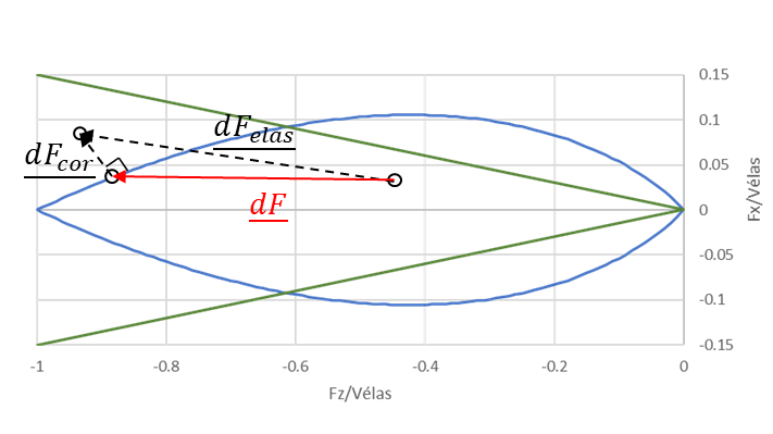
Figure 2.1-2: Illustration of the feedback on the CP criterion

2.1.4.3. If \({f}_{\mathit{CP}}\le 0\) and \({f}_{s}>0\)#

Only the mechanism of loss of load-bearing capacity is achieved, no plasticity variable related to sliding changes:

\({Q}_{\mathit{CP}}^{F}={Q}_{CP}^{O}\text{ },{U}_{\mathit{CP}}^{F}={U}_{\mathit{CP}}^{O},{v}_{z,\mathit{CP}}^{pl,F}={v}_{z,\mathit{CP}}^{pl,O}\)

The situation is solved in the same way as in § 2.1.4.2, we then look for the correction in loading \({\mathrm{d}F}^{cor}\text{ }\) and the evolution of the work-hardening variables \({\mathrm{d}Q}_{sl}\) necessary to return to the criterion, namely:

\({f}_{sl}({F}^{élas}-{\mathrm{d}F}^{cor},{Q}_{sl}^{O}+\mathrm{d}{Q}_{sl})=0\)

This equation is solved by an iterative loop until convergence, by writing in iteration k the limited expansion of this equation around point \(\text{ }({F}^{ité,k},{Q}_{sl}^{ité,k})\):

\({f}_{s}\left({F}^{élas}-{\mathrm{d}F}^{cor},{Q}_{sl}^{O}+\mathrm{d}{Q}_{sl}\right)\approx \left\{\begin{array}{c}{f}_{s}\left({F}^{ité,k},{Q}_{sl}^{ité,k}\right)\\ +{}^{T}\left(\frac{\partial {f}_{s}}{\partial F}\left({F}^{ité,k},{Q}_{sl}^{ité,k}\right)\right)\left({F}^{élas}-{\mathrm{d}F}^{cor}-{F}^{ité,k}\right)\\ +{}^{T}\left(\frac{\partial {f}_{s}}{\partial {Q}_{sl}}\left({F}^{ité,k},{Q}_{sl}^{ité,k}\right)\right)\left({Q}_{sl}^{O}+{\mathrm{d}Q}_{sl}-{Q}_{sl}^{ité,k}\right)\end{array}\right\}=0\)

Starting with the iterative loop: \(({F}^{ité,0},{Q}_{sl}^{ité,0})=({F}^{élas},{Q}_{sl}^{O})\)

The correction in loading and the evolution of work hardening can be linked to the plastic displacement increment \({\mathrm{d}U}_{sl}^{k}\) by the following relationships:

\({\mathrm{d}F}^{cor}={K}_{élas}^{O,tan}\cdot {\mathrm{d}U}_{sl}^{k}\) and \({\mathrm{d}Q}_{sl}={H}_{sl}^{O}\cdot {\mathrm{d}U}_{sl}^{k}\)

Where \({H}_{sl}^{O}\text{ }\) is calculated with the parameters at the start of the time step (see §1.2).

We assume that the plastic flow is normal to the plasticity surface, so we relate the plastic increment to the plastic flow variable \(d{\lambda }_{sl}^{k}\):

\({\mathrm{d}U}_{sl}^{k}=\frac{\partial {f}_{s}}{\partial F}\left({F}^{ité,k},{Q}_{sl}^{ité,k}\right)\mathrm{d}{\lambda }_{sl}^{k}\)

Thus we can write to obtain an approximation of the plastic flow:

\(\mathrm{d}{\lambda }_{sl}^{k}=\frac{{f}_{s}\left({F}^{ité,k},{Q}_{sl}^{ité,k}\right)+{}^{T}\left(\frac{\partial {f}_{s}}{\partial F}\left({F}^{ité,k},{Q}_{sl}^{ité,k}\right)\right)\left({F}^{élas}-{F}^{ité,k}\right)+{}^{T}\left(\frac{\partial {f}_{s}}{\partial {Q}_{sl}}\left({F}^{ité,k},{Q}_{sl}^{ité,k}\right)\right)\left({Q}_{\mathit{CP}}^{O}-{Q}_{sl}^{ité,k}\right)}{\left({}^{T}\left(\frac{\partial {f}_{s}}{\partial F}\left({F}^{ité,k},{Q}_{sl}^{ité,k}\right)\right){K}_{élas}^{O,tan}-{}^{T}\left(\frac{\partial {f}_{s}}{\partial {Q}_{sl}}\left({F}^{ité,k},{Q}_{sl}^{ité,k}\right)\right){H}_{sl}^{O}\right)\times \left(\frac{\partial {f}_{s}}{\partial F}\left({F}^{ité,k},{Q}_{sl}^{ité,k}\right)\right)}\)

si:math: `left| {f} _ {s}left ({F} ^ {alas} - {mathrm {d} F} ^ {cor}, {Q} _ {sl} ^ {O}} + {mathrm {d} {O}}} + {mathrm {d}}O}O} + {mathrm {d} Q}left ({F} ^ {O}} + {mathrm {d} Q}left) _ {sl}right) - {mathrm {d} F}} ^ {cor}, {Q} _ {sl} ^ {O}} + {mathrm {d} {O}} + {mathrm {d} Q} + {mathrm {d} Q correction;
otherwise we start the loop again with: \(\left({F}^{ité,k+1},{Q}_{sl}^{ité,k+1}\right)=\left({F}^{élas}-{\mathrm{d}F}^{cor},{Q}_{sl}^{O}+{\mathrm{d}Q}_{sl}\right)\)

After convergence of the loop at iteration « m », the plasticity parameters related to sliding are updated:

math:: {Q} _ {sl} ^ {F} = {Q} _ {F} = {Q} _ {F} = {U} _ {sl} ^ {F} = {U} _ {sl} ^ {O} ^ {O} + {mathrm {o}} + {O} + {O} + {Q} _ {O} + {Q} _ {O} + {Q} _ {O} = {O} + {Q} _ {O} + {Q} _ {O} + {Q} _ {O} + {Q} _ {O} = {O} + {Q} _ {O} = {O} + {Q} _ {O} = {O} + {Q} _ {O} = {V} U} = {V} U} = {V} U} x, s} ^ {pl, O} +left|mathrm {d} {U} _ {x, s} ^ {pl, m+1}right|text {}, {v} _ {y, s} _ {y, s}} ^ {y, s} ^ {pl, s} +left|mathrm {d} {s, s} _ {y, s} _ {y, s} _ {y, s} ^ {d} {u} _ {y} _ {y} _ {y, s}, s} ^ {pl, m+1}right|

We also recover the strength at the end of the time step:

\({F}^{F}={F}^{ité,m+1}\)

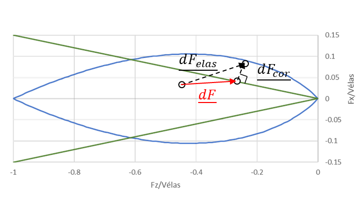
Figure 2.1-3: Illustration of the feedback on the sliding criterion

2.1.4.4. If \({f}_{\mathit{CP}}>0\) and \(>\)#

Then both plasticity mechanisms are reached. We then solve the situation in the same way as in § 2.1.4.2 and § 2.1.4.3 but by writing the two criteria instead of one, by writing the limited expansion of this equation around the point \(\text{ }\left({F}^{ité,k},{Q}_{\mathit{CP}}^{ité,k},{Q}_{sl}^{ité,k}\right)\) in iteration k:

\({f}_{\mathit{CP}}\left({F}^{élas}-{\mathrm{d}F}^{cor},{Q}_{\mathit{CP}}^{O}+\mathrm{d}{Q}_{\mathit{CP}}\right)\approx \left\{\begin{array}{c}{f}_{\mathit{CP}}\left({F}^{ité,k},{Q}_{\mathit{CP}}^{ité,k}\right)\\ +{}^{T}\left(\frac{\partial {f}_{\mathit{CP}}}{\partial F}\left({F}^{ité,k},{Q}_{\mathit{CP}}^{ité,k}\right)\right)\left(\underline{{F}^{élas}}-{\mathrm{d}F}^{cor}-{F}^{ité,k}\right)\\ +{}^{T}\left(\frac{\partial {f}_{\mathit{CP}}}{\partial {Q}_{\mathit{CP}}}\left({F}^{ité,k},{Q}_{\mathit{CP}}^{ité,k}\right)\right)\left({Q}_{\mathit{CP}}^{O}+{\mathrm{d}Q}_{\mathit{CP}}-{Q}_{CP}^{ité,k}\right)\end{array}\right\}=0\)

Starting with the iterative loop: \(({F}^{ité,0},{Q}_{\mathit{CP}}^{ité,k},{Q}_{sl}^{ité,0})=({F}^{élas},{Q}_{CP}^{O},{Q}_{sl}^{O})\)

The correction in loading and the evolution of work hardening can be linked to the plastic displacement increments \({\mathrm{d}U}_{\mathit{CP}}^{k}\) and \({\mathrm{d}U}_{sl}^{k}\) by the following relationships:

\({\mathrm{d}F}^{cor}={K}_{élas}^{O,tan}\left({\mathrm{d}U}_{\mathit{CP}}^{k}+{\mathrm{d}U}_{sl}^{k}\right)\text{ }\) and \({\mathrm{d}Q}_{\mathit{CP}}={\mathrm{I}}_{\mathrm{CP}}^{\mathrm{O}}\cdot {\mathrm{d}U}_{\mathit{CP}}^{k}\) and \({\mathrm{d}Q}_{sl}={H}_{sl}^{O}\cdot {\mathrm{d}U}_{sl}^{k}\)

We assume that the plastic flow is normal to the plasticity surface, so we relate the plastic increment to the plastic flow variables \(\mathrm{d}{\lambda }_{\mathit{CP}}^{k}\) and \(d{\lambda }_{sl}^{k}\):

\({\mathrm{d}U}_{\mathit{CP}}^{k}=\frac{\partial {f}_{\mathit{CP}}}{\partial F}\left({F}^{ité,k},{Q}_{\mathit{CP}}^{ité,k}\right)\mathrm{d}{\lambda }_{CP}^{k}\text{ }\mathrm{et}\text{ }{\mathrm{d}U}_{sl}^{k}=\frac{\partial {f}_{s}}{\partial F}\left({F}^{ité,k},{Q}_{sl}^{ité,k}\right)\mathrm{d}{\lambda }_{sl}^{k}\)

The system is thus obtained:

\(\left(\begin{array}{cc}{m}_{\mathit{CP},\mathit{CP}}& {m}_{s,\mathit{CP}}\\ {m}_{s,\mathit{CP}}& {m}_{s,s}\end{array}\right)\left(\begin{array}{c}\mathrm{d}{\lambda }_{\mathit{CP}}^{k}\\ \mathrm{d}{\lambda }_{sl}^{k}\end{array}\right)=\left(\begin{array}{c}\stackrel{~}{{f}_{\mathit{CP}}^{k}}\\ \stackrel{~}{{f}_{s}^{k}}\end{array}\right)\text{}\mathrm{ou}\text{ }M\times \mathrm{d}{\lambda }^{k}=\stackrel{~}{{f}^{k}}\)

With:

\({m}_{\mathit{CP},\mathit{CP}}=\left({}^{T}\left(\frac{\partial {f}_{\mathit{CP}}}{\partial F}\left({F}^{ité,k},{Q}_{\mathit{CP}}^{ité,k}\right)\right){K}_{élas}^{O,tan}-{}^{T}\left(\frac{\partial {f}_{\mathit{CP}}}{\partial {Q}_{\mathit{CP}}}\left({F}^{ité,k},{Q}_{\mathit{CP}}^{ité,k}\right)\right){I}_{\mathit{CP}}^{O}\right)\times \left(\frac{\partial {f}_{CP}}{\partial F}\left({F}^{ité,k},{Q}_{CP}^{ité,k}\right)\right)\)
\({m}_{s,s}=\left({}^{T}\left(\frac{\partial {f}_{s}}{\partial F}\left({F}^{ité,k},{Q}_{sl}^{ité,k}\right)\right){K}_{élas}^{O,tan}-{}^{T}\left(\frac{\partial {f}_{s}}{\partial {Q}_{sl}}\left({F}^{ité,k},{Q}_{sl}^{ité,k}\right)\right){H}_{sl}^{O}\right)\times \left(\frac{\partial {f}_{s}}{\partial F}\left({F}^{ité,k},{Q}_{sl}^{ité,k}\right)\right)\)
\({m}_{s,CP}={}^{T}\left(\frac{\partial {f}_{\mathit{CP}}}{\partial F}\left({F}^{ité,k},{Q}_{\mathit{CP}}^{ité,k}\right)\right){K}_{élas}^{O,tan}\left(\frac{\partial {f}_{s}}{\partial F}\left({F}^{ité,k},{Q}_{sl}^{ité,k}\right)\right)\)
\(\stackrel{~}{{f}_{\mathit{CP}}^{k}}={f}_{\mathit{CP}}\left({F}^{ité,k},{Q}_{\mathit{CP}}^{ité,k}\right)+{}^{T}\left(\frac{\partial {f}_{\mathit{CP}}}{\partial F}\left({F}^{ité,k},{Q}_{\mathit{CP}}^{ité,k}\right)\right)\left({F}^{élas}-{F}^{ité,k}\right)+{}^{T}\left(\frac{\partial {f}_{CP}}{\partial {Q}_{\mathit{CP}}}\left({F}^{ité,k},{Q}_{\mathit{CP}}^{ité,k}\right)\right)\left({Q}_{\mathit{CP}}^{O}-{Q}_{\mathit{CP}}^{ité,k}\right)\)
\(\stackrel{~}{{f}_{s}^{k}}={f}_{s}\left({F}^{ité,k},{Q}_{sl}^{ité,k}\right)+{}^{T}\left(\frac{\partial {f}_{s}}{\partial F}\left({F}^{ité,k},{Q}_{sl}^{ité,k}\right)\right)\left({F}^{élas}-{F}^{ité,k}\right)+{}^{T}\left(\frac{\partial {f}_{s}}{\partial {Q}_{sl}}\left({F}^{ité,k},{Q}_{sl}^{ité,k}\right)\right)\left({Q}_{sl}^{O}-{Q}_{sl}^{ité,k}\right)\)

The reversal of this system makes it possible to obtain the plastic multipliers \(\mathrm{d}{\lambda }_{\mathit{CP}}^{k}\) and \(\mathrm{d}{\lambda }_{sl}^{k}\). We deduce \({\mathrm{d}U}_{\mathit{CP}}^{k}\), \({\mathrm{d}U}_{sl}^{k}\), \({\mathrm{d}F}^{cor}\), \(\mathrm{d}{Q}_{sl}\) and \({\mathrm{d}Q}_{CP}\) from this, we reassess the failure criteria:

si:Math: left| {f} _ {mathit {CP}}}left ({F} ^ {elas} - {mathrm {d} F} ^ {cor}, {Q} _ {Q} _ {mathit {CP} _ {mathit {CP}} _ {mathit {CP}}}right)Q} _ {mathit {CP}} _ {mathit {CP}} _ {mathit {CP}} _ {mathit {CP}} _ {mathit {CP}} _ {mathit {CP}} _ {mathit {CP}} _ {mathit {CP}} _ {mathit {CP}} _ {mathit {CP}} _ {mathit {CP}}} mathrm {error} and:math: left| {f} | {f} _ {s}left ({F} ^ {elas} - {mathrm {d} F} ^ {cor}, {Q} _ {sl} _ {sl} _ {d} Q} + {mathrm {d}} Q} + {mathrm {d} Q}} _ {sl}right)right|lemathrm {error}

so we have reached the convergence of the correction, we then check that \(\mathrm{d}{\lambda }_{\mathit{CP}}^{k}>0\) and \(\mathrm{d}{\lambda }_{sl}^{k}>0\), otherwise:

If \(\mathrm{d}{\lambda }_{\mathit{CP}}^{k}<0\), then it means that failure is not reached by load-bearing capacity and the calculation is performed as a single sliding criterion (see § 1.2);

If \(\mathrm{d}{\lambda }_{sl}^{k}<0\), then it means that failure by sliding is not achieved and the calculation is performed as a single load-bearing capacity criterion (see § 1.3);

otherwise we start the loop again with:

\(\left({F}^{ité,k+1},{Q}_{\mathit{CP}}^{ité,k+1},{Q}_{sl}^{ité,k+1}\right)=\left({F}^{élas}-{\mathrm{d}F}^{cor},{Q}_{\mathit{CP}}^{O}+{\mathrm{d}Q}_{\mathit{CP}},{Q}_{sl}^{O}+{\mathrm{d}Q}_{sl}\right)\)

After convergence of the loop at iteration « m », the plasticity parameters related to load-bearing capacity and sliding are updated:

math:: {Q} _ {sl} ^ {F} = {Q} _ {F} = {Q} _ {F} = {U} _ {sl} ^ {F} = {U} _ {sl} ^ {O} ^ {O} + {mathrm {o}} + {O} + {O} + {Q} _ {O} + {Q} _ {O} + {Q} _ {O} = {O} + {Q} _ {O} + {Q} _ {O} + {Q} _ {O} + {Q} _ {O} = {O} + {Q} _ {O} = {O} + {Q} _ {O} = {O} + {Q} _ {O} = {V} U} = {V} U} = {V} U} x, s} ^ {pl, O} +left|mathrm {d} {U} _ {x, s} ^ {pl, m+1}right|text {}, {v} _ {y, s} _ {y, s}} ^ {y, s} ^ {pl, s} +left|mathrm {d} {d} {s, s} _ {y, s} _ {y, s} ^ {d} {u} _ {y, s} ^ {d} {u} _ {y} _ {y, s}, s} ^ {pl, m+1}right|
math:: {Q} _ {mathit {CP}}} ^ {CP}} ^ {F} = {Q} _ {mathit {CP}}} ^ {U} _ {mathit {CP}}} ^ {F}} ^ {F} = {F} = {U} = {U} _ {U} _ {mathit {CP}}} ^ {O} + {mathrm {d} U} _ {mathit {CP}}} ^ {m}, {v} _ {z, CP} ^ {pl, F} ^ {pl, F} = {v} _ {z, CP} ^ {pl, O} +left|mathrm {d} {U} {U} _ {z, F} _ {z, F} _ {z, F}} = {v} _ {pl, CP} ^ {pl, m+1}right|

We also recover the strength at the end of the time step:

\({F}^{F}={F}^{ité,m+1}\)

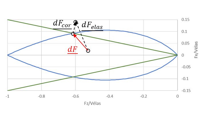
Figure 2.1-4: Illustration of the feedback on both criteria

2.1.4.5. Convergence parameters#

The convergence parameters of the iterative loop used in [§ 2.1.4.2], [§ 2.1.4.3] and [§ 2.1.4.4] can be entered by the user via the keywords ITER_INTE_MAXI and RESI_INTE_RELA associated with the keyword factor COMPORTEMENT:

The convergence criterion of the loop is associated with the convergence tolerance RESI_INTE_RELA and the elastic limit of the law of behavior \(>\), such as

\(\mathrm{error}={V}_{lim}\times \text{RESI\_INTE\_RELA}\)

The number of iterations in this loop cannot exceed ITER_INTE_MAXI (which must be greater than 0). If the number of iterations is exceeded, the behavior algorithm returns an error and a time step subdivision is applied if this option is activated (via DEFI_LIST_INST). It is also strongly recommended to activate the automatic division of the time step in order to ensure the convergence of the calculation.
It is also verified in the calculation that the value of isotropic work hardening is accurate, namely at iteration k that:

\(\begin{array}{c}{R}^{k}=\left({V}_{ult}-{V}_{lim}\right)\left(\frac{{v}_{z,CP}^{pl,k}}{{v}_{z,\mathit{CP}}^{pl,k}+{v}_{r,\mathit{CP}}^{pl}}\right)\end{array}\)

Otherwise we perform an additional iteration by replacing in \({I}_{\mathit{CP}}^{O}\), the term \(\frac{\partial R}{\partial {U}_{z,\mathit{CP}}^{pl}}\) by:

\(\frac{\Delta R}{\Delta {U}_{z,\mathit{CP}}^{pl}}=\frac{\left({V}_{ult}-{V}_{lim}\right)\left(\frac{{v}_{z,\mathit{CP}}^{pl,k}}{{v}_{z,\mathit{CP}}^{pl,k}+{v}_{r,\mathit{CP}}^{pl}}\right)-{R}^{O}}{{U}_{z,\mathit{CP}}^{pl,k}-{U}_{z,\mathit{CP}}^{pl,O}}\)

2.1.4.6. Managing inflection points#

The load-bearing capacity criterion has two inflection points and the sliding criterion has one inflection point. At the level of these inflection points, the resolution methods in the preceding paragraphs are not sufficient, it is then necessary to separate the criterion into several sub-criteria in order to be able to converge on the inflection points as shown in the figure below:

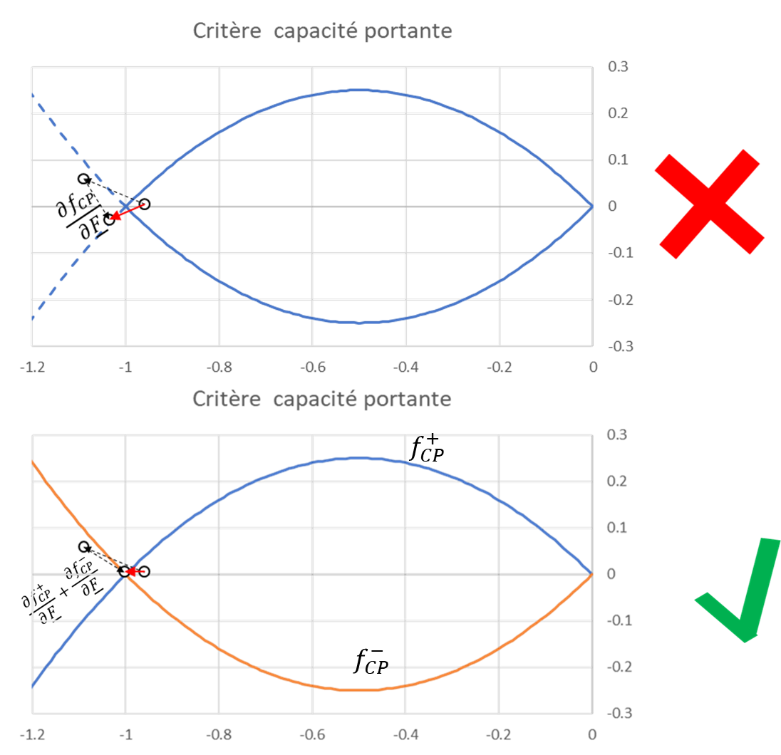
Figure 2.1-5: Illustration of the decomposition into two sub-criteria at the inflection points

Thus, to manage the load-bearing capacity criterion, it is necessary to consider 4 sub-criteria:

The normal criterion:

\({f}_{\mathit{CP}}^{+++\text{}}=-{F}_{z}-\overline{V}{\left(1+\frac{\sqrt{{\overline{{F}_{x}}}^{2}+{\overline{{F}_{y}}}^{2}}}{{F}_{z}}\right)}^{3}\left(1+\delta \left(\overline{{M}_{x}^{O}}\right)\frac{2\overline{{M}_{x}}}{{L}_{y}{F}_{z}}\right)\left(1+\delta \left(\overline{{M}_{y}^{O}}\right)\frac{2\overline{{M}_{y}}}{{L}_{x}{F}_{z}}\right)\)

With: \(\text{ }\overline{{F}_{x}}={F}_{x}-{R}_{h,x},\text{ }\overline{{F}_{y}}={F}_{y}-{R}_{h,y},\text{ }\overline{{M}_{x}}={M}_{x}-{R}_{m,x},\text{ }\overline{{M}_{y}}={M}_{y}-{R}_{m,y},\text{ }\)

\(\delta \left(\overline{{M}_{x}^{O}}\right)=\{\begin{array}{c}+1\text{ }\mathrm{si}\text{ }\overline{{M}_{x}^{O}}={M}_{x}^{O}-{R}_{r,x}^{O}>0\text{ }\text{au début du pas de temps}\\ -1\text{ }\mathrm{si}\text{ }\overline{{M}_{x}^{O}}={M}_{x}^{O}-{R}_{r,x}^{O}<0\text{ }\text{au début du pas de temps}\end{array}\)

\(\delta \left(\overline{{M}_{y}^{O}}\right)=\{\begin{array}{c}+1\text{ }\mathrm{si}\text{ }\overline{{M}_{y}^{O}}={M}_{y}^{O}-{R}_{r,y}^{O}>0\text{ }\text{au début du pas de temps}\\ -1\text{ }\mathrm{si}\text{ }\overline{{M}_{y}^{O}}={M}_{y}^{O}-{R}_{r,y}^{O}<0\text{ }\text{au début du pas de temps}\end{array}\)

The criterion with horizontal force reversal:

\({f}_{\mathit{CP}}^{H-\text{}}=-{F}_{z}-\overline{V}{\left(1-\frac{\sqrt{{\overline{{F}_{x}}}^{2}+{\overline{{F}_{y}}}^{2}}}{{F}_{z}}\right)}^{3}\left(1+\delta \left(\overline{{M}_{x}^{O}}\right)\frac{2\overline{{M}_{x}}}{{L}_{y}{F}_{z}}\right)\left(1+\delta \left(\overline{{M}_{y}^{O}}\right)\frac{2\overline{{M}_{y}}}{{L}_{x}{F}_{z}}\right)\)

The criterion with moment reversal according to x:

\({f}_{\mathit{CP}}^{Mx-\text{}}=-{F}_{z}-\overline{V}{\left(1+\frac{\sqrt{{\overline{{F}_{x}}}^{2}+{\overline{{F}_{y}}}^{2}}}{{F}_{z}}\right)}^{3}\left(1-\delta \left(\overline{{M}_{x}^{O}}\right)\frac{2\overline{{M}_{x}}}{{L}_{y}{F}_{z}}\right)\left(1+\delta \left(\overline{{M}_{y}^{O}}\right)\frac{2\overline{{M}_{y}}}{{L}_{x}{F}_{z}}\right)\)

The criterion with moment reversal according to y:

\({f}_{\mathit{CP}}^{My-\text{}}=-{F}_{z}-\overline{V}{\left(1+\frac{\sqrt{{\overline{{F}_{x}}}^{2}+{\overline{{F}_{y}}}^{2}}}{{F}_{z}}\right)}^{3}\left(1+\delta \left(\overline{{M}_{x}^{O}}\right)\frac{2\overline{{M}_{x}}}{{L}_{y}{F}_{z}}\right)\left(1-\delta \left(\overline{{M}_{y}^{O}}\right)\frac{2\overline{{M}_{y}}}{{L}_{x}{F}_{z}}\right)\)

To manage the slippage criterion, it is necessary to consider 2 sub-criteria:

The normal criterion:

\({f}_{s}^{+\text{}}=\sqrt{{\left({F}_{x}-{q}_{hx}\right)}^{2}+{\left({F}_{y}-{q}_{hy}\right)}^{2}}+{F}_{z}\mathrm{tan}({\varphi }_{inter})-{c}_{inter}{A}^{\text{'}}\)

The criterion with horizontal force reversal:

\({f}_{s}^{-\text{}}=-\sqrt{{\left({F}_{x}-{q}_{hx}\right)}^{2}+{\left({F}_{y}-{q}_{hy}\right)}^{2}}+{F}_{z}\mathrm{tan}({\varphi }_{inter})-{c}_{inter}{A}^{\text{'}}\)

The system is then solved as a multi-criteria in the same way as in § 2.1.4.4.

2.1.4.7. Managing convergence at the origin#

The writing of the load-bearing capacity criterion and the resolution of the associated plastic flow indicated in § 1.3 is only possible if:

\(>\)
\(>\)
\(>\)

Otherwise, the elastic pull has exceeded the definition limit of the failure criterion and there is a discrepancy in the resolution algorithm as illustrated in the figure below:

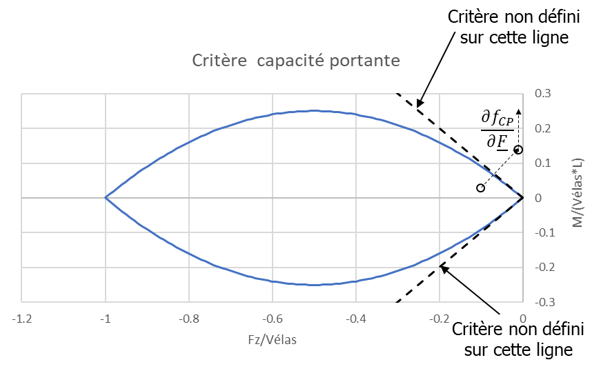
Figure 2.1-6: Illustration of the decomposition into two sub-criteria at the inflection points

To avoid this discrepancy, it would suffice to reduce the time step to prevent the elastic pull from being too far from the criterion and to ensure the convergence of the algorithm, which is done in the code. However, at the origin level \(>\), the border between the criterion and the convergence limit zone is very/too weak and it would take a step of time tending towards 0 to ensure convergence. To solve the problem, the criterion is linearized starting with \(>\):

In the case of a load that is mainly rotating \(>\);
In the case of a mainly horizontal load \(>\);

The load-bearing capacity criterion is then transformed into 3 linearized criteria:

According to horizontal force:

\({f}_{\mathit{CP},lin}^{H}={\left(1-\frac{{l}_{in}}{\left(1-\frac{2\left({M}_{x}-{R}_{m,x}\right)}{{l}_{in}{L}_{y}\left({V}_{lim}+R\right)}\right)\left(1-\frac{2\left({M}_{y}-{R}_{m,y}\right)}{{l}_{in}{L}_{x}\left({V}_{lim}+R\right)}\right)}\right)}^{\frac{1}{3}}{F}_{z}+\sqrt{{\left({F}_{x}-{R}_{h,x}\right)}^{2}+{\left({F}_{y}-{R}_{h,y}\right)}^{2}}\)

Depending on the moment in x:

math:: `{f} _ {mathit {CP}, lin}, lin} ^ {Mx} =left (1-frac {{l} _ {in}} {{left (1-frac {2frac {22sqrt {sqrt {left {{left ({F}}) {left ({F} _ {y} - {R} _ {h, y}right)}} ^ {2}}}} {{l}}} {{l} _ {y}left ({V} _ {lim} +Rright)}right)}right)}right)}} ^ {3}}} ^ {3}}left (1-frac {2}left (1-frac {2}left ({M} _ {y}left)} {{l} _ {in} {L} _ {x}left ({V} _ {V} _ {lim} +Rright)}right) {L} _ {y} {F} _ {z} +2left| {m}}} +2left| {M} _ {z} +2left| {M} _ {z} +2left| {M} _ {z} +2left| {M} _ {x} - {R} _ {m, x} {F} _ {f} _ {z} +2left| {M} _ {z} +2left| {M} _ {z} +2

Depending on the moment in time:

math:: `{f} _ {mathit {CP}, lin}, lin} ^ {My} =left (1-frac {{l} _ {in}} {{left (1-frac {2frac {2sqrt {{left} {{left ({left ({F}}) {F} _ {y} - {R} _ {h, y}right)}} ^ {2}}}} {{l}}} {{l} _ {y}left ({V} _ {lim} +Rright)}right)}right)}right)}} ^ {3}}} ^ {3}}left (1-frac {2}left (1-frac {2}left ({M} _ {x} - {M} _ {lim} +Rright)}}right)} {{l} _ {in} {L} _ {x}left ({V}}left ({V} _ {lim} +Rright)}right) {L} _ {x} {F} _ {f} _ {z} +2left| {M}} +2left| {M} _ {z} +2left| {M} _ {z} +2left| {M} _ {y} - {R} _ {m, y} {F} _ {f} _ {z} +2left| {M} _ {z} +2left| {M} _ {z} +2left| {M}

In order to manage the inflection point in \(>\), these sub-criteria are themselves subdivided into two:

For the criterion linearized according to horizontal force:

\({f}_{\mathit{CP},lin}^{H+\text{}}={\left(1-\frac{{l}_{in}}{\left(1-\frac{2\left({M}_{x}-{R}_{m,x}\right)}{{l}_{in}{L}_{y}\left({V}_{lim}+R\right)}\right)\left(1-\frac{2\left({M}_{y}-{R}_{m,y}\right)}{{l}_{in}{L}_{x}\left({V}_{lim}+R\right)}\right)}\right)}^{\frac{1}{3}}{F}_{z}+\sqrt{{\left({F}_{x}-{R}_{h,x}\right)}^{2}+{\left({F}_{y}-{R}_{h,y}\right)}^{2}}\)

\(\mathrm{et}\text{ }{f}_{\mathit{CP},lin}^{H-\text{}}={\left(1-\frac{{l}_{in}}{\left(1-\frac{2\left({M}_{x}-{R}_{m,x}\right)}{{l}_{in}{L}_{y}\left({V}_{lim}+R\right)}\right)\left(1-\frac{2\left({M}_{y}-{R}_{m,y}\right)}{{l}_{in}{L}_{x}\left({V}_{lim}+R\right)}\right)}\right)}^{\frac{1}{3}}{F}_{z}-\sqrt{{\left({F}_{x}-{R}_{h,x}\right)}^{2}+{\left({F}_{y}-{R}_{h,y}\right)}^{2}}\)

For the criterion linearized according to the moment in x:

\({f}_{\mathit{CP},lin}^{Mx+\text{}}=\left(1-\frac{{l}_{in}}{{\left(1-\frac{2\sqrt{{\left({F}_{x}-{R}_{h,x}\right)}^{2}+{\left({F}_{y}-{R}_{h,y}\right)}^{2}}}{{l}_{in}{L}_{y}\left({V}_{lim}+R\right)}\right)}^{3}\left(1-\frac{2\left({M}_{y}-{R}_{m,y}\right)}{{l}_{in}{L}_{x}\left({V}_{lim}+R\right)}\right)}\right){L}_{y}{F}_{z}+2\delta \left(\overline{{M}_{x}^{O}}\right)\left({M}_{x}-{R}_{m,x}\right)\)

\(\mathrm{et}\text{ }{f}_{\mathit{CP},lin}^{Mx-\text{}}=\left(1-\frac{{l}_{in}}{{\left(1-\frac{2\sqrt{{\left({F}_{x}-{R}_{h,x}\right)}^{2}+{\left({F}_{y}-{R}_{h,y}\right)}^{2}}}{{l}_{in}{L}_{y}\left({V}_{lim}+R\right)}\right)}^{3}\left(1-\frac{2\left({M}_{y}-{R}_{m,y}\right)}{{l}_{in}{L}_{x}\left({V}_{lim}+R\right)}\right)}\right){L}_{y}{F}_{z}-2\delta \left(\overline{{M}_{x}^{O}}\right)\left({M}_{x}-{R}_{m,x}\right)\)

For the criterion linearized according to the moment in y:

\({f}_{\mathit{CP},lin}^{My+\text{}}=\left(1-\frac{{l}_{in}}{{\left(1-\frac{2\sqrt{{\left({F}_{x}-{R}_{h,x}\right)}^{2}+{\left({F}_{y}-{R}_{h,y}\right)}^{2}}}{{l}_{in}{L}_{y}\left({V}_{lim}+R\right)}\right)}^{3}\left(1-\frac{2\left({M}_{x}-{R}_{m,x}\right)}{{l}_{in}{L}_{y}\left({V}_{lim}+R\right)}\right)}\right){L}_{x}{F}_{z}+2\delta \left(\overline{{M}_{y}^{O}}\right)\left({M}_{y}-{R}_{m,y}\right)\)

\(\mathrm{et}\text{ }{f}_{\mathit{CP},lin}^{My-\text{}}=\left(1-\frac{{l}_{in}}{{\left(1-\frac{2\sqrt{{\left({F}_{x}-{R}_{h,x}\right)}^{2}+{\left({F}_{y}-{R}_{h,y}\right)}^{2}}}{{l}_{in}{L}_{y}\left({V}_{lim}+R\right)}\right)}^{3}\left(1-\frac{2\left({M}_{x}-{R}_{m,x}\right)}{{l}_{in}{L}_{y}\left({V}_{lim}+R\right)}\right)}\right){L}_{x}{F}_{z}-2\delta \left(\overline{{M}_{y}^{O}}\right)\left({M}_{y}-{R}_{m,y}\right)\)

The system is then solved as a multi-criteria in the same way as in § 2.1.4.4.

2.2. Determining the tangent matrix#

2.2.1. Input data#

In addition to the parameters of the law of behavior, we have as input the variables obtained at the end or at the beginning of the time step (we will therefore not use the F or O notation) whose calculation is presented in § 2.1:

global strength: \(F={}^{T}\left({F}_{x},{F}_{y},{F}_{z},{M}_{x},{M}_{y},{M}_{z}\right)\)
sliding work hardening variables: \({Q}_{sl}={}^{T}\left({q}_{hx},{q}_{hy}\right)\)
plastic sliding movement: \({U}_{sl}={}^{T}\left({U}_{x,s}^{pl},{U}_{y,s}^{pl},{U}_{z,s}^{pl},{\theta }_{x,s}^{pl},{\theta }_{y,s}^{pl}\right)\)
work-hardening variables in load bearing capacity: \({Q}_{CP}={}^{T}\left({R}_{h,x},{R}_{h,y},R\text{ },{R}_{m,x},\text{ }{R}_{m,y}\right)\)
plastic displacement in bearing capacity: \({U}_{\mathit{CP}}={}^{T}\left({U}_{x,\mathit{CP}}^{pl},{U}_{y,\mathit{CP}}^{pl},{U}_{z,\mathit{CP}}^{pl},{\theta }_{x,\mathit{CP}}^{pl},{\theta }_{y,\mathit{CP}}^{pl}\right)\)
internal variables in sliding and load-bearing capacity: \({v}_{x,s}^{pl}\), \({v}_{y,s}^{pl}\) and \({v}_{z,\mathit{CP}}^{pl}\)
As well as all their associated differentials \(\mathrm{d}F,\text{}\mathrm{d}{Q}_{sl},\text{ }\mathrm{d}{Q}_{\mathit{CP}},\mathrm{d}{U}_{sl},\text{ }\mathrm{d}{U}_{\mathit{CP}}\)
the internal variable \({d}^{état}\) which indicates which criteria were met during the calculation of the loading increment, which makes it possible to have all the criteria reached taking into account the management of convergence at the origin (§ 2.1.4.7) and the sub-criteria for the management of inflection points (§ 2.1.4.6).

2.2.2. Composition of the tangent matrix#

2.2.2.1. If \(>\)#

Then no plasticity mechanism is achieved which corresponds to § 2.1.4.1, the foundation is in the elastic domain. From the global force \(F\), the tangent elastic stiffness in rotation according to x \({K}_{\mathit{rx},\mathit{rx}}^{tan}\) and y \({K}_{\mathit{ry},\mathit{ry}}^{tan}\) are calculated with the formulation seen in [§ 1.4] so we obtain the tangent elastic stiffness matrix which is in the case of \(>\) the tangent matrix:

\(K={K}_{élas}^{tan}=\left(\begin{array}{cccccc}{K}_{\mathit{xx}}^{ini}& 0& 0& 0& 0& 0\\ 0& {K}_{\mathit{yy}}^{ini}& 0& 0& 0& 0\\ 0& 0& {K}_{\mathit{zz}}^{ini}& 0& 0& 0\\ 0& 0& 0& {K}_{\mathit{rx},\mathit{rx}}^{tan}& 0& 0\\ 0& 0& 0& 0& {K}_{\mathit{ry},\mathit{ry}}^{tan}& 0\\ 0& 0& 0& 0& 0& {K}_{\mathit{rz},\mathit{rz}}^{ini}\end{array}\right)\)

2.2.2.2. If \(>\)#

Reading \({d}^{état}\text{ }\) allows you to know which failure criteria were met during the previous loading phase. We note here that there were \({n}_{s}\) sub-criteria for failure by slip reached (taking into account the possible inflection point presented in § 2.1.4.6) noted \({f}_{s}^{i\in ⟦1,ns⟧}\) (with \({\lambda }_{s}^{i}\) the associated plastic multiplier) and \({n}_{\mathit{CP}}\) sub-criteria for failure by bearing capacity reached (taking into account the points of inflection presented in § 2.1.4.6) as well as the management of the convergence originally presented in § 2.1.4.7) noted \({f}_{\mathit{CP}}^{j\in ⟦1,{n}_{\mathit{CP}}⟧}\) (with \({\lambda }_{\mathit{CP}}^{j}\) the associated plastic multiplier).

For each sub-criterion, we have:

\({f}_{s}^{i}=0,\text{ }\mathrm{d}{f}_{s}^{i}={}^{T}\left(\frac{\partial {f}_{s}^{i}}{\partial F}\right)\mathrm{d}F+{}^{T}\left(\frac{\partial {f}_{s}^{i}}{\partial {Q}_{sl}}\right)\mathrm{d}{Q}_{sl}=0\text{ }\mathrm{et}\text{ }{f}_{\mathit{CP}}^{j}=0,\text{}\mathrm{d}{f}_{\mathit{CP}}^{j}={}^{T}\left(\frac{\partial {f}_{\mathit{CP}}^{j}}{\partial F}\right)\mathrm{d}F+{}^{T}\left(\frac{\partial {f}_{\mathit{CP}}^{j}}{\partial {Q}_{\mathit{CP}}}\right)\mathrm{d}{Q}_{\mathit{CP}}=0\)

By establishing the following relationships:

\(\mathrm{d}F={K}_{élas}^{tan}\cdot \mathrm{d}{U}_{élas}={K}_{élas}^{tan}\left(\mathrm{d}U-\mathrm{d}{U}_{s}-\mathrm{d}{U}_{\mathit{CP}}\right),\text{ }\mathrm{d}{Q}_{sl}={H}_{sl}\cdot \mathrm{d}{U}_{sl},\text{ }\mathrm{d}{Q}_{\mathit{CP}}={I}_{\mathit{CP}}\cdot \mathrm{d}{U}_{\mathit{CP}}\)

We note the plastic flows:

\(\mathrm{d}{U}_{sl}=\sum _{i=1}^{i={n}_{s}}\frac{\partial {f}_{s}^{i}}{\partial F}\mathrm{d}{\lambda }_{sl}^{i}\text{ }\mathrm{et}\text{ }\mathrm{d}{U}_{CP}=\sum _{j=1}^{j={n}_{CP}}\frac{\partial {f}_{\mathit{CP}}^{j}}{\partial F}\mathrm{d}{\lambda }_{\mathit{CP}}^{j}\)

We arrive at the following system:

\(\left(\begin{array}{cc}{M}_{sl,sl}^{K}& {M}_{sl,\mathit{CP}}^{K}\\ {}^{T}\left({M}_{sl,\mathit{CP}}^{K}\right)& {M}_{\mathit{CP},\mathit{CP}}^{K}\end{array}\right)\left(\begin{array}{c}{\mathrm{d}\mathrm{\lambda }}_{\mathrm{s}\mathrm{l}}^{\mathrm{i}\in \left(1\mathrm{,}\mathrm{n}\mathrm{s}\right)}\text{ }\\ {\mathrm{d}\lambda }_{CP}^{j\in \left(1,{n}_{CP}\right)}\text{ }\end{array}\right)=\left(\begin{array}{c}{}^{T}\left(\frac{\partial {f}_{s}^{i\in \left(1,ns\right)}}{\partial F}\right)\\ {}^{T}\left(\frac{\partial {f}_{\mathit{CP}}^{j\in \left(1,{n}_{\mathit{CP}}\right)}}{\partial F}\right)\end{array}\right){K}_{élas}^{tan}\mathrm{d}U\text{ }\mathrm{ou}\text{ }{M}^{K}\mathrm{d}\lambda ={}^{T}\left(\frac{\partial f}{\partial F}\right){K}_{élas}^{tan}\mathrm{d}U\)

With:

\({\left({M}_{sl,sl}^{K}\right)}_{(i,j)\in {⟦1,ns⟧}^{2}}={}^{T}\left(\frac{\partial {f}_{s}^{i}}{\partial F}\right){K}_{élas}^{tan}\left(\frac{\partial {f}_{s}^{j}}{\partial F}\right)-{}^{T}\left(\frac{\partial {f}_{s}^{i}}{\partial {Q}_{sl}}\right){H}_{sl}\left(\frac{\partial {f}_{s}^{j}}{\partial F}\right)\)
\({\left({M}_{sl,\mathit{CP}}^{K}\right)}_{(i,j)\in \left(1,{n}_{s}\right)\times \left(1,{n}_{\mathit{CP}}\right)}={}^{T}\left(\frac{\partial {f}_{s}^{i}}{\partial F}\right){K}_{élas}^{tan}\left(\frac{\partial {f}_{\mathit{CP}}^{j}}{\partial F}\right)\)
\({\left({M}_{\mathit{CP},\mathit{CP}}^{K}\right)}_{(i,j)\in {\left(1,{n}_{\mathit{CP}}\right)}^{2}}={}^{T}\left(\frac{\partial {f}_{\mathit{CP}}^{i}}{\partial F}\right){K}_{élas}^{tan}\left(\frac{\partial {f}_{\mathit{CP}}^{j}}{\partial F}\right)-{}^{T}\left(\frac{\partial {f}_{\mathit{CP}}^{i}}{\partial {Q}_{\mathit{CP}}}\right){I}_{\mathit{CP}}\left(\frac{\partial {f}_{CP}^{j}}{\partial F}\right)\)
For simplification \(\left(\begin{array}{c}{\mathrm{d}\lambda }_{sl}^{i\in \left(1,ns\right)}\text{ }\\ {\mathrm{d}\lambda }_{\mathit{CP}}^{j\in \left(1,{n}_{\mathit{CP}}\right)}\text{ }\end{array}\right)=\mathrm{d}\lambda\) and \(\left(\begin{array}{c}{}^{T}\left(\frac{\partial {f}_{s}^{i\in \left(1,ns\right)}}{\partial F}\right)\\ {}^{T}\left(\frac{\partial {f}_{\mathit{CP}}^{j\in \left(1,{n}_{\mathit{CP}}\right)}}{\partial F}\right)\end{array}\right)={}^{T}\left(\frac{\partial f}{\partial F}\right)\)

This system is subsequently reversed:

\({\left({M}^{K}\right)}^{-1}={\left(\begin{array}{cc}{M}_{sl,sl}^{K}& {M}_{sl,\mathit{CP}}^{K}\\ {}^{T}\left({M}_{sl,\mathit{CP}}^{K}\right)& {M}_{\mathit{CP},\mathit{CP}}^{K}\end{array}\right)}^{-1}=\left(\begin{array}{cc}{S}_{sl,sl}^{K}& {S}_{sl,\mathit{CP}}^{K}\\ {}^{T}\left({S}_{sl,\mathit{CP}}^{K}\right)& {S}_{\mathit{CP},\mathit{CP}}^{K}\end{array}\right)={S}^{K}\)

The expression for plastic flow is thus obtained:

\(\mathrm{d}\lambda ={S}^{K}{}^{T}\left(\frac{\partial f}{\partial F}\right){K}_{élas}^{tan}\mathrm{d}U\)

Starting from the relationship between force and elastic displacement:

\(\mathrm{d}F={K}_{élas}^{tan}\mathrm{d}{U}_{élas}={K}_{élas}^{tan}\left(\mathrm{d}U-\sum _{i=1}^{i=ns}\frac{\partial {f}_{s}^{i}}{\partial F}\mathrm{d}{\lambda }_{sl}^{i}-\sum _{j=1}^{j={n}_{\mathit{CP}}}\frac{\partial {f}_{\mathit{CP}}^{j}}{\partial F}\mathrm{d}{\lambda }_{\mathit{CP}}^{j}\right)={K}_{élas}^{tan}\left(\mathrm{d}U-\left(\frac{\partial f}{\partial F}\right)\mathrm{d}\lambda \right)\)

So we can write:

\(\mathrm{d}F=\left({K}_{élas}^{tan}-{K}_{élas}^{tan}\left(\frac{\partial f}{\partial F}\right){S}^{K}{}^{T}\left(\frac{\partial f}{\partial F}\right){K}_{élas}^{tan}\right)\mathrm{d}U\)

After inverting \({M}^{K}\), the program therefore returns the tangent plastic matrix:

\({K}^{tan}={K}_{élas}^{tan}-{K}_{élas}^{tan}\left(\frac{\partial f}{\partial F}\right){S}^{K}{}^{T}\left(\frac{\partial f}{\partial F}\right){K}_{élas}^{tan}\)