2. Variational formulation of the damage problem#
2.1. Case of a generic law (explained here in traction)#
Two equivalent approaches can be used to describe the process of damaging a fragile isotropic material. On the one hand, it is possible to derive the law of damage within the framework of generalized standard materials. In this case, it is necessary to define the free energy of the system as well as a dissipation potential. The flow rule then establishes the evolution of the internal variables.
As for the description of damage, all you need is a scalar variable. The previous description is simplified and can be reduced to a variational problem under the stress of increased damage [bib2].
To define a behavior law with a damage gradient, it is therefore sufficient to express the total free energy density (elastic+dissipation) as a function of the deformation tensor \(\varepsilon\) and the damage variable \(0\le a\le 1\). The spatial distribution of the damage is then given by a field \(a(x)\). The free energy density generally takes the following form:
\(\Phi (\varepsilon ,a)=A(a)w(\varepsilon )+\omega (a)+c/2{(\nabla a)}^{2}\) eq 2.1-1
Here \(c\) is the nonlocality parameter (C_ GRAD_VARI) \(w(\varepsilon )\) the elastic deformation energy, \(\omega (a)\) the dissipation energy, and \(A(a)\) the stiffness function. \(a=0\) corresponds to healthy material and \(a=1\) corresponds to completely damaged material: \(A(1)=\mathrm{0,}A(0)=1\). The evolution problem is now a simple Helmholtz free energy minimization problem \(F\equiv \int \Phi (\varepsilon ,a)d\Omega\) under \(\dot{a}\ge 0\) constraint [1] _ .
\({\mathrm{min}}_{(\varepsilon ,a)}F(\varepsilon ,a),\text{où}F(\varepsilon ,a)=\int \left[\Phi (\varepsilon ,a)\right]d\Omega\)
where we replace \(w(\varepsilon )=\varepsilon :E:\varepsilon /2\) using the Hooke tensor definition. Two equations derive from the variational minimization problem: \(\delta F(\varepsilon ,a)/\delta \varepsilon =0\) [2] _ and \(\delta F(\varepsilon ,a)/\delta a\ge 0\). The inequality in the second equation is related to the presence of imposed constraints. These two equations must be satisfied everywhere in integration domain \(\Omega\). They are completed by a Kuhn-Tucker \(\dot{a}\cdot \delta F(\varepsilon ,a)/\delta a=0\) coherence equation. On edges \(\partial \Omega\) we get an additional normality condition \(\nabla a\cdot n=0\), where \(n\) is a normal-vector. Finally, the damage variable and its gradient must be continuous within the integration domain to achieve the minimum of the functional in question (see [bib2,4] for more details).
2.2. Behavioral relationships#
The link between the variational formulation and the usual laws of evolution is direct. The condition of the material is characterized by deformation \(\varepsilon\) and damage \(a\), ranging between 0 and 1. The stress-strain relationship is defined, which remains elastic, and the stiffness is affected by the damage:
\(\sigma =\delta F(\varepsilon ,a)/\delta \varepsilon =A(a)E:\varepsilon\) eq 2.2-1
with \(E\) the Hooke tensor. The evolution of damage, which is always increasing, is governed by the following threshold function:
\(f(\varepsilon ,a)=-\delta \Phi (\varepsilon ,a)/\delta a=-\frac{1}{2}A\text{'}(a)\varepsilon :E:\varepsilon -\omega \text{'}(a)+c\Delta a\) eq 2.2-2
The coherence condition then takes on its usual form:
\(f(\varepsilon ,a)\le 0\dot{a}\ge 0\dot{a}f(\varepsilon ,a)=0\) eq 2.2-3
Two particularities of this formulation are noted. First, the threshold function is non-local because of the presence of the damaging Laplacian. Then, the absence of flow conditions is justified by the double role of damage \(a\), on the one hand it is presented as an internal evolution variable, on the other hand it fulfills the mission of the Lagrange parameter \(\lambda \equiv a\).
We also see the advantage of presenting damage laws in their variational form. It suffices to describe the total free energy density (eq.2.1-1), which includes dissipation, to completely define the law of evolution.
2.3. Identifying law ENDO_CARRE#
In law ENDO_CARRE, the stiffness and dissipation functions are chosen as follows:
\(A(a)={(1-a)}^{2},\omega (a)=\mathrm{ka}\)
The mechanical parameters of the law are three in number. On the one hand, the Young’s modulus \(E\) and the Poisson’s ratio \(\nu\) which determine the Hooke tensor by:
\({E}^{-1}\cdot \sigma =\frac{1+\nu }{E}\sigma -\frac{\nu }{E}(\text{tr}\sigma )\text{Id}\) eq 2.3-1
as well as \(k\), which defines the softening behavior and the characteristic width of the damage band. By noting \({\sigma }_{y}\) the peak stress and \(l\) the internal length characteristic of the size of the damaged area, the following relationships are established:
\(k=\frac{{\sigma }_{y}^{2}}{E},c=E{l}^{2}\)
The parameters of the model are directly given under the keywords factors ECRO_LINE (SY) and NON_LOCAL (C_ GRAD_VARI) of the operator DEFI_MATERIAU. As for \(E\) and \(\nu\), they are classically given under the keyword factor ELAS or ELAS_FO. Note that the parameter D_ SIGM_EPSI is not used here although it must be given a value in the command file, because it is in mandatory status. The ECRO_LINE keyword was used to avoid duplicating objects in DEFI_MATERIAU that all refer to the limit constraint.
Example: |
\(\begin{array}{}E=30\text{GPa,}\nu =0.2\\ {\sigma }_{y}=3\text{MPa}\end{array}\) |
|
Below is answer \(\sigma (\varepsilon )\) obtained in 1 point, based on the parameters chosen as an example:
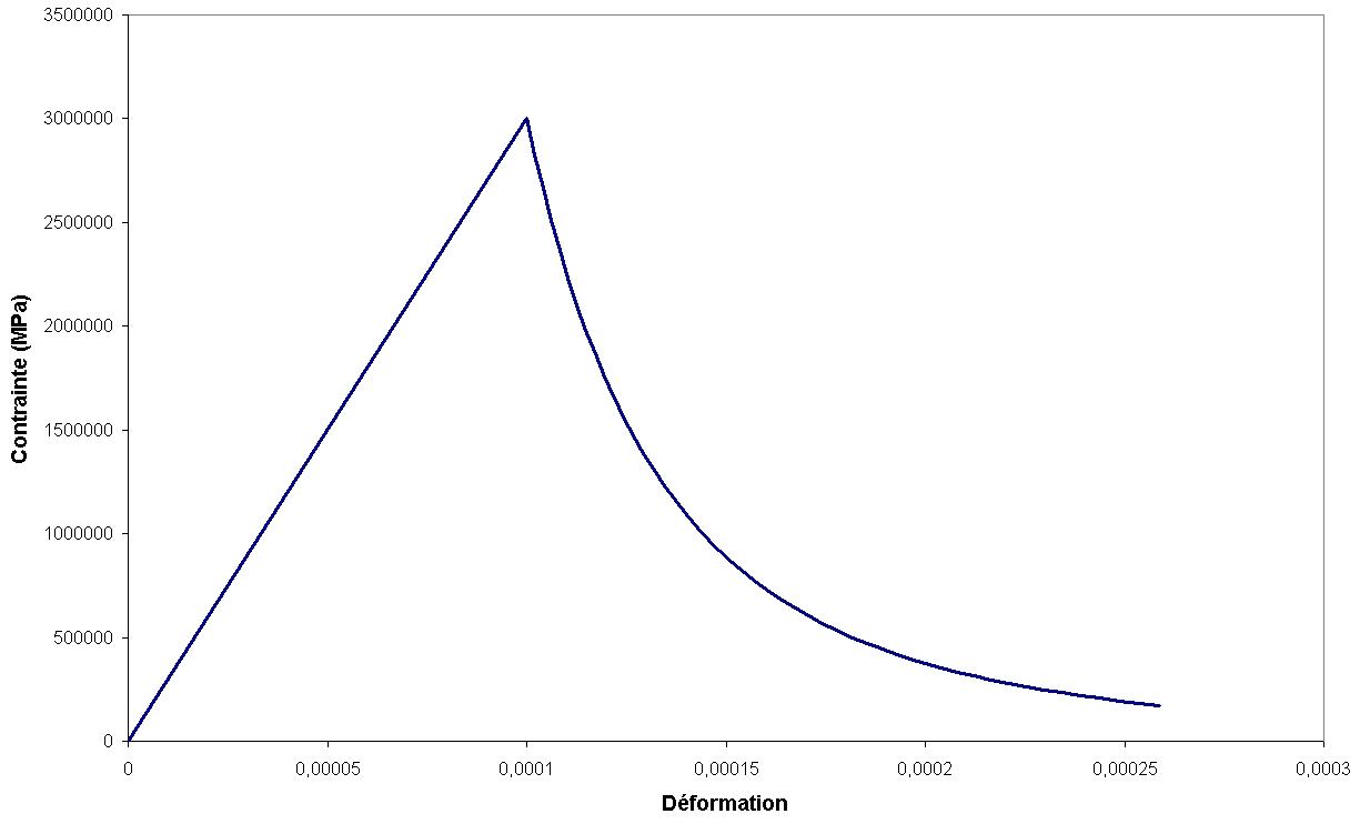
Figure 1: Stress-strain response
As long as critical stress \({\sigma }_{y}\) is not reached, the response is linear elastic and the damage is zero. Once this value is reached, a decrease in stress is observed as a function of deformation in \({\varepsilon }^{-3}\). This is explained by the quadratic decrease in stiffness as a function of damage.
2.4. Compression behavior#
In the case of traction (« crack opening »), the elastic energy is corrected by a quadratic factor corresponding to the loss of stiffness (see eq 2.2.1). In the case of compression (« closure »), only the part associated with the deviatory deformation tensor is corrected. The constraint field can then be written in the form:
\(\sigma ={(1-a)}^{2}({k}_{2}\mathrm{tr}(\varepsilon )H\mathrm{tr}(\varepsilon )+2\mu {\varepsilon }_{D})+{k}_{2}\mathrm{tr}(\varepsilon )H\mathrm{tr}(-\varepsilon )\)
Where \({\varepsilon }_{D}\) is the deviatoric tensor of the deformations, \(H\) the Heaviside function and \({k}_{2}=\lambda +\frac{2\mu }{3}\), with \(\lambda\) and \(\mu\) the Lamé coefficients.
As the stresses have to be finite, the trace of the strain tensor is checked. This makes it possible to avoid significant deformations in the direction of the forces, contrary to what is done for traction. Taking into account the loss of stiffness affected to the deviatory part, it is however possible to obtain sliding jumps in the direction of shear. This behavior prohibits interpenetration but therefore allows damage by shear.
The criterion is also amended as follows:
\(f(\varepsilon ,a)=-\frac{1}{2}A\text{'}(a)\left[2\mu {\varepsilon }_{D}:{\varepsilon }_{D}+H(\mathrm{tr}(\varepsilon )){k}_{2}{(\mathrm{tr}(\varepsilon ))}^{2}\right]-\omega \text{'}(a)+c\Delta a\)
This model is very well representative of the behavior of a concrete structure when the damage occurs in the form of a strip. This is always the case in 2D. However, in order to have good compression behavior in 3D, in the event that the damage no longer occurs in the form of a band, the damage should no longer be caused to be carried out on the diverter, but on the rotational one.
2.5. Description of internal variables#
There are two internal variables:
\(\mathrm{VI}(1)\) damage \(a\)
\(\mathrm{VI}(2)\) indicator \(\chi\)