2. Writing and hypotheses

This algorithm, due to C.Miehe; N.Apel and M.Lambrecht [13] is based on an energetic formulation and the stiffness matrix is provided in [13].

2.1. Kinematic elements

The cinematic elements in the continuous case can be found for example in [3]. Here we will focus on the case directly discretized in time making it possible to define the quantities used in the formalism presented in this document. We consider a closed initial continuous domain \({\Omega }_{0}\subset {ℝ}^{3}\), each point of which is identified by its coordinates \(X\in {\Omega }_{0}\), undergoing a deformation field \(\varphi\) causing it to pass into the configuration \(\Omega\):

(2.1)\[ \ varphi\ mathrm {:} {\ Omega} _ {0} _ {0}\ to\ Omega\ subset {492} ^ {3}\]

The coordinates of this point will be noted \(x\in \Omega\) in the current configuration.

Since the deformation evolves over time, we actually define, through temporal discretization, a family of \({\varphi }_{n}\) fields each corresponding to an instant \({t}_{n}\) in the history of evolution of the domain.

In the case of the large deformations formalism treated here, it is necessary to introduce four configurations for the domain and its evolution (cf. Figure 1): the initial reference configuration \({\Omega }_{0}\) (i.e. for which the deformations are zero), the configuration \({\Omega }_{n}\) at the beginning of the current time step \({t}_{n\text{+}1}={t}_{n}+\Delta t\), the configuration \({\Omega }_{n\text{+}1}\) at the end of this time step, and a configuration in the middle of the time step, \({\Omega }_{n\text{+}\frac{1}{2}}\), formalism being integrated with a middle point rule.

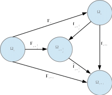
Figure 1: Required configurations and transformation gradients

From these configurations, the displacement fields and the transformation gradients are defined in order to go from one to the other. The quantities that make it possible to go from the initial configuration to a given configuration are noted in uppercase \((U,\mathrm{F})\) and the quantities connecting two deformed configurations together are noted in lower case \((u,\mathrm{f})\). Table 1 summarizes the various quantities and their expressions.

Starting configuration	Arrival configuration	Displacement	Transformation gradient
\({\Omega }_{0}\)	\({\Omega }_{n}\)	\({U}_{n}\)	\({\mathrm{F}}_{n}={\mathrm{I}}_{d}+{\mathrm{grad}}_{0}{U}_{n}\)
\({\Omega }_{0}\)	\({\Omega }_{n\text{+}1}\)	\({U}_{n+1}\)	\({\mathrm{F}}_{n+1}={\mathrm{I}}_{d}+{\mathrm{grad}}_{0}{U}_{n+1}\)
\({\Omega }_{0}\)	\({\Omega }_{n\text{+}\frac{1}{2}}\)		\({\mathrm{F}}_{n+\frac{1}{2}}=\frac{1}{2}\left({\mathrm{F}}_{n}+{\mathrm{F}}_{n+1}\right)\)
\({\Omega }_{n}\)	\({\Omega }_{n\text{+}\frac{1}{2}}\)		\({\mathrm{f}}_{n+\frac{1}{2}}={I}_{d}+\frac{1}{2}{\mathrm{grad}}_{n}u\) \({\mathrm{f}}_{n+\frac{1}{2}}={\mathrm{F}}_{n+\frac{1}{2}}\cdot {\mathrm{F}}_{n}^{-1}\) \({\mathrm{f}}_{n+\frac{1}{2}}=\frac{1}{2}\left({\mathrm{f}}_{n}+{\mathrm{I}}_{d}\right)\)
\({\Omega }_{n}\)	\({\Omega }_{n+1}\)	\(u\)	\({\mathrm{f}}_{n+1}={I}_{d}+{\mathrm{grad}}_{n}u\) \({\mathrm{f}}_{n+1}={\mathrm{F}}_{n+1}\cdot {\mathrm{F}}_{n}^{-1}\) \({\mathrm{f}}_{n+1}=\Delta \mathrm{F}\)
\({\Omega }_{n+\frac{1}{2}}\)	\({\Omega }_{n+1}\)		\({\stackrel{̃}{\mathrm{f}}}_{n+\frac{1}{2}}={\mathrm{f}}_{n+1}\cdot {\mathrm{f}}_{n+\frac{1}{2}}^{-1}\) \({\stackrel{̃}{\mathrm{f}}}_{n+\frac{1}{2}}={\mathrm{F}}_{n+1}\cdot {\mathrm{F}}_{n+\frac{1}{2}}^{-1}\)

Table 1: summary of movements and transformation gradients

From these transformation gradients, it is possible to define deformation rates \(\mathrm{L}\):

(2.2)\[ {\ mathrm {L}} _ {°}} = {\ dot {\ mathrm {F}}}} _ {°} {\ dot {\ mathrm {F}}}}} _ {°} ^ {-1}}\]

The \(\omega\) rotation rate tensors:

(2.3)\[ {\ mathrm {d}} _ {°} =\ frac {1} {2}\ left ({\ mathrm {L}} _ {°} + {\ mathrm {L}}} _ {°}} _ {°} {°} ^ {T}\ right)\]

and the \(\mathrm{d}\) strain rate tensors:

\[\]

: label: eq-4

{omega} _ {°} =frac {1} {2} {2}left ({mathrm {L}}} _ {°} - {mathrm {L}}} _ {°} {°} {°} ^ {T}right)

with \({}_{°}\) designating the \(n\), \(n+1\), or \(n+\frac{1}{2}\) configuration. The Eulerian deformation tensor between configurations \({\Omega }_{n}\) and \({\Omega }_{n+1}\) is deduced from these definitions:

\[\]

: label: eq-5

{mathrm {e}} _ {n+1} =frac {1} {2} =left [{mathrm {I}}} _ {d} - {left ({mathrm {f}}} _ {n+1}} _ {n+1}}right)} ^ {-1}}} _ {n+1}right)} ^ {-1}right]

The deformation rate is then well linked to the Eulerian deformation:

(2.4)\[ {\ mathrm {d}} _ {n+\ frac {1} {2}}} =\ frac {1} {\ delta t} {\ stackrel {} {\ mathrm {f}}}}} _ {n+\ frac {1} {1} {2}}} ^ {2}}} ^ {2}} {-1}\ cdot {\ mathrm {e}}} {n+1}} _ {n+1}} _ {n+1}} _ {n+1}} _ {n+1}} _ {n+1}} _ {n+1}} _ {n+1}}} _ {n+1}} _ {n+1}}} _ {n+1}} _ {n+1}}} _ {n+1}}} _ {n+1}}} _ {rel {} {\ mathrm {f}}}}} _ {n+\ frac {1} {2}}\]

The last quantity to be introduced for our algorithm is the incremental displacement gradient, relative to configuration \({\Omega }_{n\text{+}\frac{1}{2}}\) and defined by:

(2.5)\[ {\ mathrm {h}} _ {n+\ frac {1} {2}}} = {\ mathrm {grad}} _ {n} u\ cdot {\ mathrm {f}}} _ {n+\ frac {1} {2}}} ^ {-1}} _ {f}}} _ {f}}} _ {f}}} _ {f}}\]

The latter makes it possible to determine the rotation rate in the same configuration by the relationship:

(2.6)\[ {\ omega} _ {n+\ frac {1} {2}}} =\ frac {1}} {2\ Delta t}\ left [{\ mathrm {h}} _ {n+\ frac {1} {2}}} - {\ mathrm {2}}}} - {\ mathrm {h}}}} _ {n+\ frac {1} {2}} _ {n+\ frac {1} {h}}} _ {n+\ frac {1} {2}} ^ {T}\ right]\]

From these kinematic elements, it is possible to define hypoelastic laws of behavior whose integration is objective in large deformations. The following paragraph presents this type of formulation of laws of behavior.

2.2. Hypo-elastoplastic laws of behavior

In this section, the phenomenological model class of plasticity (here independent of time) with hypoelasticity is considered. It constitutes an ad hoc extension of the writing of laws in small deformations, which allows a certain genericity and represents an advantage in the context of a calculation code: we will see in the next chapter that it is possible to achieve its numerical integration in a way equivalent to that of small deformations.

This class of models is in contrast to the hyperelastic class, based on the thermodynamic approach to continuous media. In this context, free energy, which can for example be considered as a function of temperature and Green-Lagrange deformation, is defined; changes in stresses and possibly internal variables result from this. For example, we can cite the case of the hyperelastic law of Signorin (cf. [4]) in elasticity and the Simo-Miehe formalism in hyperelastoplasticity (cf. [3]).

A hypo-elastoplastic law of behavior is generally constructed in five steps.

1. Like the additive decomposition of small deformations, the deformation rate \(\mathrm{d}\) is first broken down into an elastic part and a plastic part:

(2.7)\[ \ mathrm {d} = {\ mathrm {d}}} ^ {e} + {\ mathrm {d}} ^ {p}\]

1. A derivative of Kirchhoff stress \(\tau =\mathit{det}(\mathrm{F})\sigma\) is then determined by an incremental relationship that is a function of the elastic rate of deformation, with \(\stackrel{˚}{x}\) an objective derivative to be defined and \(\mathrm{C}\) the elasticity tensor. :

(2.8)\[ \ stackrel {} {\ tau} =\ mathrm {C}\ mathrm {C}\ mathrm {:}\ left [\ mathrm {d}} - {\ mathrm {d}}}} ^ {p}\ right]\]

1. A convex reversibility domain defining the allowable stress space is constructed from a function \(f\), with \(S\) the stress space and \(\mathrm{q}\) the set of \(m\) internal variables representing the kinematic work hardening of the material and \(\alpha\) the scalar variables (including isotropic work hardening):

(2.9)\[ {{\ rm E}} _ {\ tau} =\ {(\ tau,\ mathrm {q},\ alpha)\ in S\ times {390} ^ {m+1}\ mid f (\ tau,\ mathrm {q},\ alpha) ≤0\}\ mid f (\ tau,\ mathrm {q},\ alpha) ≤0\}\]

The laws of evolution of these internal variables follow a principle of normality (we only consider the associated laws of behavior here), with \(\gamma \ge 0\) the plastic multiplier, \(\frac{\partial f}{\partial \tau }(\tau ,\mathrm{q},\alpha )\) defining the direction of plastic flow and \(g(\tau ,\mathrm{q},\alpha )\) the evolution of the other internal variables:

(2.10)\[ {\ mathrm {d}} ^ {p} =\ gamma\ frac {\ partial f (\ tau,\ mathrm {q},\ alpha)} {\ partial\ tau} \ stackrel {} {q} =-\ gamma g (\ tau,\ mathrm {q},\ alpha)\]

The writing of the charge/discharge conditions, classically represented by Kuhn-Tucker, and the coherence condition:

(2.11)\[\begin{split} \ mathrm {\ {}\ begin {array} {c} {c}\ gamma\ ge 0\\ f (\ tau, q,\ alpha)\ mathrm {\ le} 0\\ gamma f (\ tau, q,\ alpha)\ gamma f (\ tau, q,\ alpha)\ gamma\ ge 0\\ ge 0\\ gamma f (\ tau, q,\ alpha)\ text {=} 0\ end {array}\end{split}\]

This class of model is therefore characterized by a strong analogy with small deformation formalisms, with an incremental writing of constraints which is not without posing some numerical integration difficulties: in fact, in order to prevent the evolution of constraints by a rigid body movement, it is necessary to have an objective integration of the equation ().

2.3. Deformation and stress tensors

The model is based on logarithmic deformation defined by:

(2.12)\[ \ mathrm {E} =\ frac {1} {2}\ mathrm {log}\ left [{\ mathrm {F}}} ^ {\ mathrm {T}}}\ mathrm {.} \ mathrm {F}\ right]\]

The definition of this term is provided in Appendix 2. The stress \(\mathrm{T}\) is defined in logarithmic space as the dual of \(\mathrm{E}\), so that the mechanical power density \({p}_{m}\) is expressed by their product \(\mathrm{T}\mathrm{:}\dot{\mathrm{E}}\). It is not a classical stress tensor, but it can be linked to the usual tensors. In fact, mechanical power is written as:

(2.13)\[ {p} _ {m} =\ mathrm {T}\ mathrm {:}\ dot {\ mathrm {E}} =\ pi\ mathrm {:}\ dot {\ mathrm {F}}\]

We get:

(2.14)\[ {p} _ {m} =\ mathrm {T}\ mathrm {:}\ dot {\ mathrm {E}} =\ mathrm {T}\ mathrm {:}\ frac {\ partial\ mathrm {F}} {\ partial\ mathrm {E}}} {\ partial\ mathrm {E}}} =\ pi\ mathrm {:}\ dot {\ mathrm {F}}} =\ mathrm {F}} =\ mathrm {T}\ mathrm {:} {\ mathrm {P}} _ {\ Pi}\ mathrm {F}}\]

With \(\Pi\) the Piola-Kirchhoff stress tensor of the first kind. What defines the tensor (fourth-order in 3D) of projection \({\mathrm{P}}_{\Pi }\):

(2.15)\[ {\ mathrm {P}} _ {\ Pi} =\ frac {\ partial\ mathrm {E}} {\ partial\ mathrm {F}}\]

So we have:

(2.16)\[ \ Pi =\ mathrm {T}\ mathrm {:} {\ mathrm {P}} _ {\ Pi}\]

The Cauchy \(\sigma\) and Kirchhoff \(\tau\) tensors will be written in the usual way:

(2.17)\[ J\ sigma =\ tau =\ Pi {\ mathrm {F}} ^ {T}\]

We can also calculate the second Piola-Kirchhoff tensor \(\mathrm{S}\) as a function of \(\mathrm{T}\):

\[\]

: label: eq-20

{p} _ {m} =mathrm {T}mathrm {:}dot {mathrm {E}} =mathrm {S}mathrm {:}dot {Delta} =mathrm {Delta} =mathrm {delta} =mathrm {:}mathrm {:}frac {1} {2}dot {mathrm {C}}}

With \(\Delta\) the Green-Lagrange strain tensor such as:

\[\]

: label: eq-21

Delta =frac {1} {2}left (mathrm {C} -mathrm {I}right) =frac {1} {2}left ({mathrm {F}}}} ^ {T}mathrm {F} -mathrm {I}right)

We have a new form of mechanical power:

(2.18)\[ {p} _ {m} =\ mathrm {T}\ mathrm {:}\ dot {\ mathrm {E}} =\ mathrm {T}\ mathrm {:}\ frac {\ partial\ mathrm {E}} {\ partial\ mathrm {E}}} {\ partial\ mathrm {E}}} =\ mathrm {C}}} =\ mathrm {C}} {S}\ mathrm {:}\ frac {1} {2}\ dot {\ mathrm {C}}\]

For the second Piola-Kirchhoff tensor \(\mathrm{S}\), we obtain:

(2.19)\[ \ mathrm {S} =\ mathrm {T}\ mathrm {:}\ mathrm {P}\]

Although the physics chosen is specific, the model makes it possible to maintain the classical additive decomposition of elastic and plastic deformations in HPP with:

(2.20)\[ {\ mathrm {E}} ^ {p} =\ frac {1} {2}\ mathrm {log} ({\ mathrm {F}}} ^ {p, T}\ mathrm {.} {\ mathrm {F}}} ^ {p})\]

Such a choice is always legitimate. It is simply the same as adopting a definition for elastic deformation. However, this proves to be consistent with a multiplicative decomposition, in the absence of rotation (coaxial situation). In addition, plastic incompressibility is ensured because:

(2.21)\[ \ mathit {tr} {\ mathrm {E}}} ^ {p} =\ mathrm {log} {J} ^ {p}\]

The elastic energy \({\psi }^{e}\) of the model also takes the same form as that of small deformations, but by adopting the concepts of stress and deformation specific to this formalism, we have:

(2.22)\[ {\ psi} ^ {e} =\ frac {1} {2} {2} {\ parallel\ mathrm {E}} - {\ mathrm {E}}\ parallel} _ {E} ^ {2} =\ frac {1} {2} =\ frac {1} {2} =\ frac {1} {2} {2}\ mathrm {2}}\ mathrm {T} - {:} {\ mathrm {C}}} _ {E} ^ {2} =\ frac {1} {2} =\ frac {1} {2} =\ frac {1} {2} =\ frac {1} {2} =\ frac {1} {2} {2}\ mathrm {2}}\ mathrm {T}:}\ mathrm {T}\]

This formulation has some advantages:

the kinematic dimension of the model is confined before and after the integration of the behavior; this was one of the main elements for the choice of the formalism; all the behavior models available in small deformations are*a priori available, provided of course that it makes physical sense (large hypoelastic deformations are well adapted to metallic behaviors, and not to concrete behaviors);

• if the model HPP admits an energetic expression, the same will be true for the large deformations model: the tangent matrix is therefore symmetric;

the only difficulty seems*a priori concentrated in the definition of logarithmic deformation, but the article [13] provides a calculation algorithm distinguishing between difficult cases (multiple eigenentities);

• the model, according to the examples presented by the authors, gives results that are very similar to those obtained by a classical formalism with multiplicative decomposition;

• the model can be extended to cases of anisotropy (initial or induced).

In addition, the article [13] provides an expression for the tangent matrix in the configuration using \(\Pi\) (called nominal); however, as it is based on a writing from Piola-Kirchhoff constraints of the first kind, non-symmetric, which is not classical and never achieved in Code_Aster, we prefer here to use the second Piola-Kirchhoff tensor to calculate the internal forces and the tangent matrix on the initial configuration, with reference to [ 15] for example.