5. Comparison with PETIT_REAC#
5.1. Approximation of large deformations by PETIT_REAC#
The principle of formulation PETIT_REAC is simply to update the geometry of the problem during Newton’s iterations (not at the end of each time step). This means that all the quantities involved in the equations of the problem are evaluated on the current configuration. Nothing else is changed compared to the case of small disturbances.
5.1.1. Cinematic description#
The kinematic description is the same as that of small disturbances. This means that a deformation increment is calculated by:
\({\Omega }_{i}\) being the updated configuration. The total deformation is then the sum of each of these linearized deformation increments, calculated on different configurations. It is therefore difficult to give it a physical meaning and it is better to use it as an indicator of the level of deformation achieved. The hypothesis of additive decomposition of deformations is applied.
5.1.2. Elastoplastic behavior relationship#
In the expression of the elastic stress-strain relationship, we saw the need to use an objective derivative: \(\stackrel{̊}{\sigma }=\mathrm{C}\mathrm{:}[\dot{\epsilon }-{\dot{\epsilon }}^{p}]\). With PETIT_REAC we replace the objective derivative with the simple time derivative: it is therefore not objective. Consequently, the use of PETIT_REAC is therefore not appropriate for large rotations but it is suitable for large deformations, under certain conditions [10]:
very small increments;
very small rotations (which implies a loading that is almost radial);
small elastic deformations in front of plastic deformations;
isotropic behavior.
5.1.3. Equilibrium and tangent matrix#
In terms of finite elements, the resolution by PETIT_REAC implies at each load step the resolution of the same non-linear system as in small deformations [11]:
With the difference that internal forces are formally calculated by:
where operator \(Q\) depends on travel. In this context, the calculation of the tangent matrix leads to:
The first term is the contribution of behavior, similar to what has been presented in small transformations, with the difference that this contribution is evaluated here in the current configuration. The second term is the contribution of geometry that is not present in small transformations.
As part of resolution PETIT_REAC, this term is not present in the calculation of the tangent matrix. So we have:
The absence of the geometric contribution in the tangent matrix can sometimes make convergence difficult.
5.2. Comparison on an example#
Formalism PETIT_REAC (cf. [6]) is based on an update of the geometry to calculate the deformation increment before integrating the behavior in an identical way to small deformations. This allows for simple treatment of large deformations, but in a very approximate, non-objective manner and which can lead to major errors.
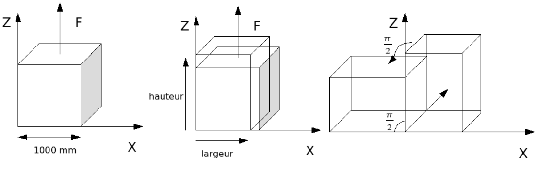
To be convinced of this, consider the alternating traction-rotation of a cube; for more details on the test, we will refer to [7] for example.
Figure 3: Example of traction and rotation of a cube
During the rotation phases, the stress must remain constant: a rigid body movement does not generate constraints (statically at least and without viscosity).
If we consider the response obtained with behavior VMIS_ISOT_LINE for deformations PETIT_REAC and GDEF_LOG, the deformation type PETIT_REAC is faulty while GDEF_LOGest is valid (and provides an answer identical to SIMO_MIEHE).