10. Parallelism and intensive computing#
10.1. Integrated operators#
The operators CALC_MODES and INFO_MODE can benefit from a first level of parallelism: that intrinsic to the linear solver MUMPS.
However, the parallel efficiency of MUMPS in a modal calculation is more limited than for other types of analyses. In general, parallel time efficiency of the order of 0.2 to 0.3 is observed for a small range of processors: from 2 to 16. Beyond that you no longer earn anything.
This can be explained in particular by:
the virtual uniqueness of certain dynamic work matrices,
a very unfavorable « number of descents/ascents to the number of factorizations » ratio,
the significant cost of the analysis phase compared to that of factorization,
a very unfavorable « time cost/memory of the linear solver »/ »time/memory cost of the modal solver » ratio.
For more technical and functional information, you can consult the documentation [R6.02.03], [U4.50.01] and [U2.08.03/06].
In order to improve in terms of performance, it is proposed to break down the initial calculation into more efficient and more accurate sub-calculations: this is the subject of one of the functionalities of the CALC_MODES operator with OPTION =” BANDE “and a list of n>2 values given under CALC_FREQ =_F (FREQ), detailed in the following paragraph. In addition, this algorithmic rewriting of the problem shows two levels of parallelism that are more relevant and more effective for « boosting » Code_Aster modal calculations.
10.2. Operator CALC_MODES, option “BANDE” split into sub-bands#
To deal effectively with large modal problems (in terms of mesh size and/or number of modes sought), it is recommended to use the CALC_MODES operator with the “BANDE” option divided into sub-bands. It breaks down the modal calculation of a standard GEP (symmetric and real), into a succession of independent, less expensive, more robust and more accurate sub-calculations.
Just sequentially, the gains can be noteable: factors 2 to 5 in time, 2 or 3 in peak RAM and 10 to 104 on the average error of the modes.
In addition, its multi-level parallelism, by reserving around sixty processors, can provide additional gains of the order of 20 in time and 2 in peak RAM (cf. tables 10-1). And this, without loss of precision, or restriction of scope and with the same numerical behavior.
perf016a test case (N=4M, 50 modes) splitting into 8 sub-bands |
Time elapsed |
Memory peak RAM |
1 processor |
5524s |
16.9GB |
8 processors |
1002s |
19.5Go |
32 processors |
643s |
13.4GB |
division into 4 sub-bands |
||
1 processor |
3569s |
17.2GB |
4 processors |
1121s |
19.5GB |
16 processors |
663s |
12.9GB |
Seismic study (N=0.7M, 450 modes) splitting into 20 sub-bands |
Time elapsed |
Memory peak RAM |
1 processor |
5200s |
10.5GB |
20 processors |
407s |
12.1GB |
80 processors |
270s |
9.4GB |
division into 5 sub-bands |
||
1 processor |
4660s |
8.2GB |
5 processors |
1097s |
11.8GB |
20 processors |
925s |
9.5GB |
Figures-Tables 10-1a/b. Some test results of CALC_MODES parallel with the default settings (+ SOLVEUR =” MUMPS “en IN_COREet * RENUM =” QAMD “) .
Code_Aster v11.3.11 on machine IVANOE (1 or 2 MPI processes per node) .
The principle of CALC_MODES [U4.52.02] with the “BAND” option divided into sub-bands, is based on the fact that the calculation and memory costs of modal algorithms depend more than linearly on the number of modes sought. So, as with domain decomposition |R6.01.03], we’re going to break down the search for hundreds of modes into more reasonable sized packages.
A package of the order of forty modes seems to be a sequential empirical optimum. At the same time, we can continue to improve performances by going down to fifteen.
The example in Figure 10-2 thus illustrates a global CALC_MODES calculation in the band
\(\mathrm{[}{\mathit{freq}}_{\mathit{min}},{\mathit{freq}}_{\mathit{max}}\mathrm{]}\)
which is often advantageously replaced by ten CALC_MODES calculations targeted at equivalent contiguous sub-bands
\(\mathrm{[}{\mathit{freq}}_{1}\mathrm{=}{\mathit{freq}}_{\mathit{min}},{\mathit{freq}}_{2}\mathrm{]},\mathrm{[}{\mathit{freq}}_{\mathrm{2,}}{\mathit{freq}}_{3}\mathrm{]},\mathrm{...}\mathrm{[}{\mathit{freq}}_{\mathrm{10,}}{\mathit{freq}}_{11}\mathrm{=}{\mathit{freq}}_{\mathit{max}}\mathrm{]}\).
On the other hand, this type of decomposition makes it possible to:
reduce robustness problems,
improve and homogenize modal errors.
In practice, this modal operator dedicated to HPC is broken down into four main steps:
Modal precalibration (via INFO_MODE) of sub-bands configured by the user:
So potentially, a loop of nb_freq independent calculations on each modal frequency position (cf. [R5.01.04]).
Effective modal calculation (via CALC_MODES + OPTION =” BANDE “+ CALC_FREQ =_F (TABLE_FREQ)) of the modes contained in each non-empty sub-band (by sharing the modal calibrations from step 1):
So potentially, a loop of nb_sbande_nonempty < nb_freq independent calculations.
Post-verification with a Sturm test on the extreme limits of the calculated modes (via INFO_MODE):
So potentially, a loop of 2 independent calculations.
Post-treatments on all the modes obtained: normalization (via NORM_MODE) and filtering (via EXTR_MODE).
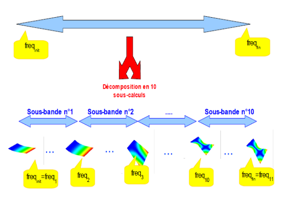
Figure 10-2. Principle of decomposition of the calculations of CALC_MODES with the option “ BANDE “divided into sub-bands.
In parallel, each of the calculation steps can identify at least one level of parallelism:
The first two by distributing the calculations for each sub-band over the same number of processor packages.
The third, by distributing the modal positions of the terminals of the verification interval over two processor packages.
The fourth step, which is inexpensive, remains sequential.
If the number of processors and the settings allow it (in particular, if we use the linear solver MUMPS), we can use a second level of parallelism.
Figure 10-3 illustrates a modal calculation seeking to take advantage of 40 processors by breaking down the initial calculation into ten search sub-bands. Each benefits from the support of 4 MUMPS occurrences for the inversions of linear systems intensively required by modal solvers.
For an exhaustive presentation of this multi-level parallelism, its challenges and some technical and functional details, you can consult the documentation [R5.01.04], [U4.52.01/02] and [U2.08.06].
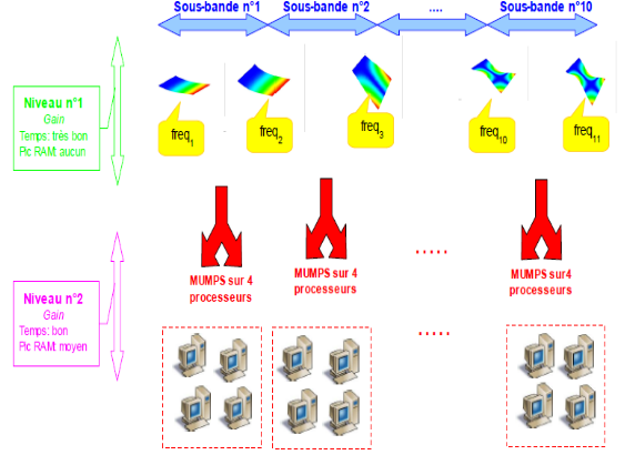
Figure 10-3. Example of two levels of parallelism in the INFO_MODE of pre-processing
and in the loop of sub-bands of CALC_MODES .
Distribution on nb_proc=4*0 processors with a division into 10 sub-bands*
(parallelism called « 10x4 ») .
Here we use the linear solver MUMPS and the parallelism setting by default (“COMPLET”) .
Notes:
In parallel MPI, the main steps concern the distribution of tasks and their communications. For CALC_MODES with the “BANDE” option divided into sub-bands, the distribution is done in the macro python as well as in the fortran. The two communicate through hidden keywords: PARALLELISME_MACRO. But all MPI calls are restricted to only the F77/F90 layers.
The global communications of the first level, those of the values and eigenvectors, are carried out at the end of the modal calculation on each sub-band. At an intermediate level, between the simple communication of linear algebra results (of the type of what is done around MUMPS/PETSc) and the communication of Aster data structures in Python after filtering (optimal in terms of performance but much more complicated to implement).
The ideal would have been to be able to balance the frequency sub-bands empirically to limit the load imbalances linked to the distribution of modes by sub-bands and those linked to the modal calculation itself. It would thus have been possible to provide 2, 4 or 8 sub-band calculations per processor. This would also make it possible to benefit from the gains of the decomposition of the macro calculation, even on a few processors. Unfortunately, computer contingencies for manipulating potentially empty user concepts did not make it possible to validate this more ambitious scenario.