3. background#
3.1. Problem#
We consider the generalized modal problem (GEP)
Find \((\lambda ,U)\) such as \(Au=\lambda Bu,u\ne 0\) (3.1-1)
where \(A\) and \(B\) are matrices with real or complex coefficients, symmetric or not (in structure and/or in values). In mechanics, this type of problem corresponds in particular to:
The study of the free vibrations of an undamped and non-rotating structure. For this structure, we look for the smallest eigenvalues or those that are in a given range to know if an exciting force can create a resonance. In this standard case, the matrix \(A\) is the stiffness matrix, noted \(\mathrm{K}\), real and symmetric (possibly increased by the geometric rigidity matrix marked \({K}_{g}\), if the structure is prestressed) and \(B\) is the mass or inertia matrix denoted by \(M\) (symmetric real). The eigenvalues obtained are the squares of the pulsations associated with the frequencies sought.
The system to be solved can be written as: \((K+{K}_{g})u={\omega }^{2}Mu\) where \(\omega =2\pi f\) is the pulsation, \(f\) the natural frequency and \(u\) the associated natural displacement vector. The \((\omega ,u)\) clean fashions are real.
In the presence of hysteretic damping, \(\mathrm{K}\) becomes complex symmetric. So clean modes are potentially complex and mismatched.
On the other hand, if \(K\) and/or \(M\) remain real but possibly not symmetric [6] _ , the modes proper are either real or in pairs \((\lambda ,\stackrel{ˉ}{\lambda })\).
This type of problem is activated by the keyword TYPE_RESU =” DYNAMIQUE “.

A / B |
Symmetric real |
Symmetric real |
Non-symmetric real |
Complex |
Symmetric real |
Most common case no restrictions on methods; Real fashions. |
Real or complex modes \((\lambda ,\stackrel{ˉ}{\lambda })\). |
Untreated case |
|
Non-symmetric real |
OPTION among (“BANDE”, “”, “”, “CENTRE”, “”, “PLUS_PETITE”, “PLUS_GRANDE”, “TOUT”) with SOLVEUR_MODAL =_F (METHODE =” SORENSEN “or” QZ “); Real modes or complexes \((\lambda ,\stackrel{ˉ}{\lambda })\). |
Real or complex modes \((\lambda ,\stackrel{ˉ}{\lambda })\). |
Untreated case |
|
Symmetric complex |
OPTION among (“BANDE”, “”, “”, “CENTRE”, “”, “PLUS_PETITE”, “PLUS_GRANDE”, “TOUT”) with SOLVEUR_MODAL =_F (METHODE =” SORENSEN “or” QZ “); Real, complex, any modes, or \((\lambda ,\stackrel{ˉ}{\lambda })\). |
Untreated case |
Untreated case |
|
Other complexes (Hermitian, non-symmetric…) |
Untreated case |
Untreated case |
Untreated case |
Untreated case |
Table 1. Scope of use of the operator CALC_MODES according to the search criterion and the analysis algorithm, according to the properties of the GEP matrices.
The linear buckling mode research. In the framework of linearized theory, assuming a priori that stability phenomena are suitably described by the system of equations obtained by assuming the linear dependence of the displacement on the critical load level, the search for the buckling mode \(u\) associated with this critical load level \(\lambda\), comes down to a generalized problem with the eigenvalues of the form: \((\mathrm{K}+\lambda {\mathrm{K}}_{\mathrm{g}})\mathrm{u}\mathrm{=}0\) with \(K\) matrix of stiffness and \({K}_{g}\) geometric rigidity matrix. To fit into the « mold » of a standard GEP calculation, the code first calculates the real \((\mathrm{-}\lambda ,u)\) eigenmodes. Then he converts them to the format of a buckling calculation: \((\lambda ,\mathrm{u})\).
This type of problem is activated by the keyword TYPE_RESU =” MODE_FLAMB “. It is reserved for real symmetric GEPs (otherwise the code detects it and produces a fatal error).
Notes:
CALC_MODES makes it possible to automate the choice of the algorithm according to the search criterion, and to reduce the costs (CPU and memory) of a search for a large part of the spectrum (only in GEP with real modes) when looking for the modes on a global band divided into sub-bands.
The user can specify which class their calculation belongs to by initializing the TYPE_RESU keyword to “DYNAMIQUE” (by default value) or to “MODE_FLAMB”. The display of the results will then be formatted taking into account this specificity. In the first case we will talk about frequency (FREQ) while in the second, we will talk about critical load (CHAR_CRIT).
In the presence of damping and gyroscopic effects,**the study of the dynamic stability* of a structure leads to the resolution of a higher-order modal problem, called quadratic (QEP) (): \((K+i\omega C-{\omega }^{2}M)u=0\). It is solved by the two modal operators and is the subject of a specific note [Boi09].
Now that the links between structural mechanics and the resolution of generalized modal problems have been recalled, we will focus on the treatments of boundary conditions in the code and their effects on mass and stiffness matrices.
3.2. Taking into account boundary conditions#
There are two ways, when constructing stiffness and mass matrices, to take into account boundary conditions (this description in terms of dynamic problems is easily extrapolated to buckling):
double dualization, using Lagrange degrees of freedom [Pel01], makes it possible to verify
\(Cu=0\) (CLL for Linear Boundary Condition),
with \(C\) real matrix of size \(p\times n\) (\(K\) and \(M\) are of order \(n\)). It involves the manipulation of larger matrices (called « dualized ») because they incorporate these new unknowns. The dualized stiffness and mass matrices then have the form
\(\tilde{\mathrm{K}}\mathrm{=}(\begin{array}{ccc}\mathrm{K}& \beta {\mathrm{C}}^{\mathrm{T}}& \beta {\mathrm{C}}^{\mathrm{T}}\\ \beta \mathrm{C}& \mathrm{-}\alpha \mathrm{Id}& \alpha \mathrm{Id}\\ \beta \mathrm{C}& \alpha \mathrm{Id}& \mathrm{-}\alpha \mathrm{Id}\end{array})\) \(\tilde{M}=(\begin{array}{ccc}M& 0& 0\\ 0& 0& 0\\ 0& 0& 0\end{array})\)
with \(\alpha\) and \(\beta\) reals that are strictly positive (which are used to balance the terms in the matrix). The dimension of the problem has been increased by \(\mathrm{2p}\), because to the \(n\) degrees of freedom called « physical », Lagranges have been added. There are two Lagranges per linear relationship assigned to the \(p\) boundary conditions.
The zeroing of \(p\) rows and columns of the stiffness and mass matrices. This is only valid for blocking degrees of freedom (simple Dirichlet, no proportionality relationship between ddls). We cannot take into account a linear relationship and we will talk about kinematic blocking (CLB for Blocking Limit Condition). The stiffness and mass matrices become:
\(\tilde{K}=(\begin{array}{cc}\stackrel{ˉ}{K}& 0\\ 0& \mathrm{Id}\end{array})\) \(\tilde{M}=(\begin{array}{cc}\stackrel{ˉ}{M}& 0\\ 0& 0\end{array})\)
The dimension of the problem remains unchanged but it is however necessary to remove the participations of the blocked ddls from the components of the initial matrices (\(\stackrel{ˉ}{K}\) is obtained from \(K\) by eliminating the rows and columns of the ddls that are blocked; same for \(\stackrel{ˉ}{M}\)).
When limiting conditions are imposed, the number of eigenvalues (with all their multiplicities) actually involved in the physics of the phenomenon is therefore less than size \(n\) of the transformed problem:
\({n}_{\mathit{ddl}\mathrm{-}\mathit{actifs}}\mathrm{=}n\mathrm{-}\frac{3p\text{'}}{2}\text{avec}p\text{'}\mathrm{=}2p\) (double dualization),
\({n}_{\mathrm{ddl}-\mathrm{actifs}}=n-p\) (kinematic blocking).
The box below shows the display dedicated to these parameters in the message file.
THE NOMBRE OF DDL
TOTAL EST: 220 \(\to\) n
FROM LAGRANGE EST: 58 \(\to\) P”=2p
THE NOMBRE OF DDL ACTIFS EST: 133 \(\to\) nddl_actifs
Example 1. Display the size of the modal problem in the message file.
On the other hand, in modal calculation algorithms, one must ensure that the solutions belong to the admissible space. We get back to it*via* auxiliary treatments. Thus, when using kinematic blocks (CLB), it is necessary, in the various algorithms and at each iteration, to use a « positioning vector » \({\mathrm{u}}_{\mathit{bloq}}\), defined by
if \(i\) th degree of freedom is not blocked \({\mathrm{u}}_{\mathit{bloq}}(i)\mathrm{=}1\),
otherwise \({\mathrm{u}}_{\mathit{bloq}}(i)\mathrm{=}0\),
and pre-multiply each vector manipulated
\({\mathrm{u}}^{1}(i)\mathrm{=}{\mathrm{u}}^{0}(i)\mathrm{\cdot }{\mathrm{u}}_{\mathit{bloq}}(i)(i\mathrm{=}\mathrm{1...n})\mathrm{\Rightarrow }{\mathrm{u}}^{1}\)
This trick introduces the constraint of blockages throughout the algorithm and implicitly orients the search for a solution in the admissible space.
Likewise, if we use the double dualization method, we need a vector for positioning the degrees of freedom of Lagrange \({\mathrm{u}}_{\mathit{lagr}}\) defined as \({\mathrm{u}}_{\mathit{bloq}}\). It is only used when choosing the initial random vector. For this vector \({u}^{0}\) to verify the boundary conditions (CLL) we operate as follows:
\(\mathrm{\mid }\begin{array}{c}{\mathrm{u}}^{1}(i)\mathrm{=}{\mathrm{u}}^{0}(i)\mathrm{\cdot }{\mathrm{u}}_{\mathit{lagr}}(i)(i\mathrm{=}\mathrm{1...n})\\ \tilde{\mathrm{K}}{\mathrm{u}}^{2}\mathrm{=}{\mathrm{u}}^{1}\end{array}\mathrm{\Rightarrow }{\mathrm{u}}^{1}\)
On the other hand, we often include the additional constraint that this initial vector belongs to the image set of the work operator. This makes it possible to enrich the modal calculation more quickly by not being limited to the core. Thus, in the case of Lanczos and IRAM, we will take as the initial vector, not the previous \({u}^{2}\), but \({u}^{3}\) such as
\({\mathrm{u}}^{3}\mathrm{=}{(\mathrm{K}\mathrm{-}\sigma \mathrm{M})}^{\text{-1}}\mathrm{M}{\mathrm{u}}^{2}\)
Subsequently, to simplify the notations, we will step distinguish between the initial matrices and their dualized counterparts (noted with a tilde) only if necessary. Very often, they will be designated by \(A\) and \(B\) in order to be closer to the usual modal notation without relating to this or that class of problems.
3.3. Properties of matrices#
In the case (the most common) where the matrices under consideration are symmetric and have real coefficients, the cases described in the table below are listed. Matrixes can be definite positive (noted \(>0\)), semi-definite positive (\(\ge 0\)), indefinite (\(\le 0\text{ou}\ge 0\)) or even singular (\(S\)).
Free structure |
Lagranges [7] _ |
Buckling |
Fluid-structure |
||
\(A(K)\) |
|
|
|
|
|
\(B\) (resp. \(M\) or \({K}_{g}\)) |
\(>0\) |
|
|
|
Table 3.3-1. Properties of the matrices of GEP.
Since the columns in this table are mutually exclusive, in practice, a buckling problem using double Lagranges to model some of its boundary conditions, its dualized matrices (\(\tilde{K}\text{et}\tilde{{K}_{g}}\)) become potentially undefined.
This range of properties must be taken into account when choosing the « (work operator, scalar product) » pair. This framework can thus reinforce, with efficiency and transparency, the robustness and the scope of the modal calculation algorithm in all cases encountered by*Code_Aster*.
In the case where matrices are complex symmetric or real non-symmetric, we can no longer define a matrix dot product. Only then are the QZ (§9) and IRAM (§7) methods available. The first does not need this type of mechanism and, the second is « bluffed » by providing it with a « false » matrix scalar product, in fact the usual Euclidean dot product (cf. §7.5). This last trick is legitimate with IRAM, because as a variant of Arnoldi, it can work with a pair (worker operator, scalar product) that is not symmetric.
The following paragraphs will allow us to measure the impact of these properties on the generalized problem spectrum.
3.4. Properties of clean modes#
First, let’s remember that if the SEP \(\mathrm{A}\mathrm{u}\mathrm{=}\lambda \mathrm{u}\) matrix is symmetric real, then its eigenelements are real; the eigenelements of a matrix are its eigenvalues and eigenvectors. On the other hand, \(A\) being normal, its eigenvectors are orthogonal.
In the case of GEP \(\mathrm{A}\mathrm{u}\mathrm{=}\lambda \mathrm{B}\mathrm{u}\), this condition is not sufficient. So, consider the following generalized problem:
\(\left[\begin{array}{cc}1& 1\\ 1& 0\end{array}\right](\begin{array}{}{u}_{1}\\ {u}_{2}\end{array})=\lambda \left[\begin{array}{cc}1& 0\\ 0& -1\end{array}\right](\begin{array}{}{u}_{1}\\ {u}_{2}\end{array})\)
its own modes are
. \({\lambda }_{\pm }=\frac{1}{2}(1\pm i\sqrt{(3)})\text{et}{u}_{\pm }=\frac{1}{\sqrt{1+{\lambda }_{\pm }^{2}}}(\begin{array}{}-{\lambda }_{\pm }\\ 1\end{array})\)
If we add the hypothesis « one of the matrices \(A\) or \(B\) is definite positive « , then the generalized problem has its real solutions. We even have the following more precise characterization (sufficient condition).
Theorem 1
Let \(A\) and \(B\) be two real symmetric matrices. If there are \(\alpha \mathrm{\in }\mathrm{ℝ}\) and \(\beta \in ℝ\) such that \(\alpha A+\beta B\) is positively defined, then the generalized problem has its own real elements.
Proof:
This result is obtained immediately by multiplying the generalized problem by \(\alpha\) and by performing a \(\beta\) spectral shift. Then we get problem \((\alpha A+\beta B)u=(\lambda \alpha +\beta )Bu\). Since \(\alpha A+\beta B\) is positive, it has a unique Cholesky decomposition in the form \(C{C}^{T}\) with \(C\) regular matrix.
The problem is then written \({C}^{\text{-1}}B{C}^{-T}z=\mu z\) with \(z={C}^{T}u\) and \(\mu =\frac{1}{\alpha \lambda +\beta }\), which allows us to conclude, since the matrix \({C}^{\text{-1}}B{C}^{-T}\) is symmetric.
notes
This characterization is not necessary, so the generalized problem associated with matrices \(A=\mathrm{diag}(\mathrm{1,}-\mathrm{2,}-1)\) and \(B=\mathrm{diag}(-\mathrm{2,1}\mathrm{,1})\) admits a real spectrum while not meeting the condition of definite positivity.
In the case of complex and Hermitian matrices, this theorem remains valid. On the other hand, in a non-Hermitian complex (this is the case when taking into account hysteretic damping in Code_Aster), the eigenmodes can be complex: eigenvectors with complex components and any real or complex \(\lambda\) eigenvalues.
In non-symmetric real, eigenmodes can be complex: eigenvectors with complex components and \(\lambda\) real or complex eigenvalues per pair \((\lambda ,\stackrel{ˉ}{\lambda })\).
Proposal 2
If the matrices \(A\) and \(B\) are real and symmetric, the eigenvectors of the generalized problem are \(A\) and \(B\) - orthogonal, which means they verify the relationships
\(\{\begin{array}{}{u}_{i}^{T}B{u}_{j}={\delta }_{\mathrm{ij}}{a}_{j}\\ {u}_{i}^{T}A{u}_{j}={\lambda }_{j}{\delta }_{\mathrm{ij}}{a}_{j}\end{array}\)
where \({a}_{j}\) is a scalar depending on the norm of the \(j\) th eigenvector, \({\delta }_{\mathrm{ij}}\) is the Kronecker symbol, and \({u}_{j}\) is the eigenvector associated with the eigenvalue \({\lambda }_{j}\).
Proof:
Immediate for distinct eigenvalues, by writing \(\mathrm{A}\) and \(B\) - dot product between two pairs \((i,j)\) and \((j,i)\), then using the symmetry of the matrices (cf. [Imb91]).
Notes:
It is shown that the \(A\) and \(B\) - orthogonalities of eigenvectors are a consequence of the hermiticity of the matrices. They are clearly a generalization of the properties of the standard Hermitian problem (or even normal): in the case of a matrix with complex and Hermitian coefficients, the dot product under consideration is a Hermitian product.
Orthogonality with respect to matrices certainly does not mean that the eigenvectors are orthogonal for the classical Euclidean norm. This can only be the result of particular symmetries (cf. TP No. 1 [BQ00]).
This property simplifies modal recombination calculations (DYNA_TRAN_MODAL [Boy07]), when manipulating generalized stiffness and mass matrices that are diagonal. The quantities j \({k}_{j}={\lambda }_{j}{a}_{j}\) and \({m}_{j}={a}_{j}\) are called, respectively, modal stiffness and modal mass of the \(j\) th mode.
For non-Hermitian matrices, Theorem 1 is no longer true.
Knowing that trends are often real, we will now focus on estimating them.
3.5. Real spectrum estimation#
The document R5.01.04 is dedicated to this problem transversal to modal operators: INFO_MODE and CALC_MODES.
Let’s just remember that in the most common case of real modes (GEP real symmetric), the problem of counting eigenvalues is solved using the famous Sturm test (see §2.2/3.2). The situation is much less favorable when the spectrum resides in the complex plane (GEP complex or non-symmetric and QEP). In this case, only the operator INFO_MODE has an adapted method: the APM method (see §2.3/3.3). But because of its enormous calculation costs and its innovative nature, it is advisable to reserve it, for the time being, for simplified problems of small size (<104 degrees of freedom).
Now that we are in a position to count the GEP spectrum, it remains to build it! Since generic algorithms are intended for SEP, we need to transform our initial problem.
3.6. Spectral transformation#
These techniques make it possible to meet a triple objective:
identify a SEP,
Orient spectrum research,
Separate eigenvalues.
Since spectral calculation algorithms converge all the better when the (working) spectrum they deal with is separated, these techniques can be considered as preconditioning of the initial problem. They make it possible to make the separation of certain modes much more important than that of other modes, and thus to improve their convergence.
The most common of these transformations is the technique called « shift and invert » which consists in working with the operator \({\mathrm{A}}_{\sigma }\) such as:
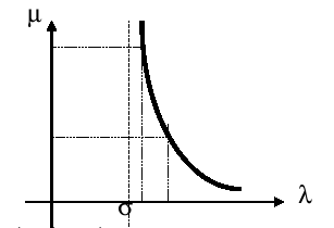
\(\text{Au}\mathrm{=}\lambda \text{Bu}\mathrm{\Rightarrow }\underset{{\mathrm{A}}_{\sigma }}{\underset{\underbrace{}}{{(\text{A}\mathrm{-}\sigma \mathrm{B})}^{\mathrm{-}1}\mathrm{B}}}\mathrm{u}\mathrm{=}\underset{\mu }{\underset{\underbrace{}}{\frac{1}{\lambda \mathrm{-}\sigma }}}\mathrm{u}\)
Figure 3.6-1. Effect of « shift and invert » on the separation of eigenvalues.
Figure 3.6-1 shows that this separation and orientation of the working spectrum in \(\mu\) is due to the particular properties of the hyperbolic function. On the other hand, it is observed that only the eigenvalues are affected by the transformation. At the end of the modal process, all you have to do is go back to the \(\lambda\) plan by changing the appropriate variable.
Notes:
Variable \(\sigma\) is usually referred to as « shift » or spectral shift.
The \({A}_{\sigma }\) work matrix must of course be invertible; this can also become one of the reasons for this discrepancy (see §6.5).
As a reminder, it should be noted that with a complex shift, several scenarios are possible:
Work completely in complex arithmetic,
In real arithmetic, by isolating the real and imaginary contributions of \({\mathrm{A}}_{\sigma }\), for example via work operators
\({A}_{\sigma }^{+}\mathrm{=}\text{Re}({A}_{\sigma })\mathrm{\Rightarrow }{\mu }^{+}\mathrm{=}\frac{1}{2}(\frac{1}{\lambda \mathrm{-}\sigma }+\frac{1}{\lambda \mathrm{-}\stackrel{ˉ}{\sigma }})\),
\({A}_{\sigma }^{\mathrm{-}}\mathrm{=}\text{Im}({A}_{\sigma })\mathrm{\Rightarrow }{\mu }^{\mathrm{-}}\mathrm{=}\frac{1}{\mathrm{2i}}(\frac{1}{\lambda \mathrm{-}\sigma }\mathrm{-}\frac{1}{\lambda \mathrm{-}\stackrel{ˉ}{\sigma }})\).
Each of these approaches has its pros and cons. For the QEP of*Code_Aster* [Boi09], this is the first approach that was chosen for Sorensen (METHODE =” SORENSEN “+ APPROCHE =” COMPLEXE “). The second is reserved for other approaches: METHODE =” SORENSEN “or” TRI_DIAG “+ APPROCHE =” REEL”/”IMAGINAIRE”).
notes
This choice of the work operator is inseparable from that of the (nickname) -scalar product. It makes it possible to move towards this or that algorithm and can thus influence the robustness of the calculation.
Other classes of spectral transformations exist. For example, Cayley’s method, with a double shift (\({\sigma }_{\mathrm{1,}}{\sigma }_{2}\)), allows you to select the eigenvalues located to the right of a vertical axis.
\(\underset{{A}_{\sigma }}{\underset{\underbrace{}}{{(\mathrm{A}\mathrm{-}{\sigma }_{1}\mathrm{B})}^{\text{-1}}(\mathrm{A}\mathrm{-}{\sigma }_{2}\mathrm{B})}}\mathrm{u}\mathrm{=}\underset{\mu }{\underset{\underbrace{}}{\frac{\lambda \mathrm{-}{\sigma }_{2}}{\lambda \mathrm{-}{\sigma }_{1}}}}\mathrm{u}\)
The next paragraph will summarize the above in the overall flowchart for solving a generalized Code_Aster modal problem.
3.7. Implementation in Code_Aster#
The process of a modal calculation in Code_Aster can be broken down into four phases. The following paragraphs detail them.
3.7.1. Determining the shift#
The first operation consists in determining the shift as well as some parameters of the problem. This is done more or less transparently depending on the calculation option chosen by the user:
OPTION =” SEPARE “or “AJUSTE” =>the shift is determined by the first phase of the algorithm and the number of natural modes sought by frequency band (provided by the Sturm criterion) is limited by NMAX_FREQ.
OPTION =” PROCHE “=>the shift is set by the user and the number of natural modes is equal to the number of shifts.
OPTION =” PLUS_PETITE “=> the shift is zero and the number of modes is set to NMAX_FREQ.
OPTION =” BANDE “=>leshift is equal to the middle of the band set by the user and the number of modes is determined by the Sturm criterion.
OPTION =” CENTRE “=> the shift is set by the user and the number of natural modes is set by NMAX_FREQ.
Notes:
This phase is not about the QZ algorithm. Indeed, the latter calculates the entire spectrum of GEP. It is just after the modal calculation that the user’s wishes are taken into account (OPTION =” BANDE “or” CENTRE “or” PLUS_PETITE “or” PLUS_GRANDE “or” TOUT “) to select the desired modes.
For a GEP with complex modes (\(\mathrm{K}\) complex symmetric or non-symmetric matrices), only the options” CENTRE “,” PLUS_PETITE “,” PLUS_GRANDE “,” TOUT “are available (with Sorensen and QZ).
3.7.2. Factorization of dynamic matrices#
In the second pre-processing phase, we factory [Boi08] « dynamic » matrices of the type \(Q(\sigma ):=A-\sigma B\) *.**That is to say, we decompose the dynamic matrix :math:`Q(sigma )` into a product of particular matrices (triangular, diagonal) that are easier to handle to solve linear systems of type :math:`Q(sigma )x=y`. In symmetric, the decomposition is of the form :math:`Q(sigma )=LD{L}^{T}`, in non-symmetric, we have :math:`Q(sigma )=LU`*, ** with \(U\), \(L\) and \(D\), respectively, upper triangular, lower and diagonal.
Once this numerical factorization (expensive) has been carried out, the resolution of other linear systems comprising the same matrix but with a different second member (multiple second member problem) is very fast.
This scenario is end:
each time the**Sturm test* is implemented. That is to say for certain scenarios in phase 1 of shift selection (OPTION =” SEPARE “/” AJUSTE “or” BANDE “) and in preparation for post-verification phase 4 when counting real eigenvalues (GEP with real and symmetric matrices only).
when you have to manipulate a work matrix that includes an inverse. For example in the case of Lanczos or IRAM (OPTION among [“BANDE”, “CENTRE”, “”, “PLUS_”,” TOUT “] + SOLVEUR_MODAL =_F (METHODE =” TRI_DIAG”/””/”SORENSEN”)), we are interested in. \({A}_{\sigma }={(A-\sigma B)}^{-1}B\) With the inverse power method (OPTION =” SEPARE “/” AJUSTE “/” PROCHE “), it is \({A}^{\sigma }={(A-\sigma B)}^{-1}\). The two other approaches, Bathe & Wilson or QZ (OPTION among [“BANDE”, “”, “CENTRE”, “PLUS_ “,” TOUT “]*+ SOLVEUR_MODAL =_F (METHODE =” JACOBI” /”QZ “)) are not concerned with this preliminary factorization of a work matrix.
Notes:
This factorization is also subject to the same hazards as the Sturm criterion when the shift is close to an eigenvalue. The same offsets are then carried out according to algorithm 1 of R5.01.04.
When this pre-processing phase uses algorithm 5 from R5.01.04 and NMAX_ITER_SHIFT is reached, the calculation produces an alarm if it is a factorization for the Sturm test (risk of numerical instabilities), a fatal error if we try to factor the working matrix (risk of false results).
When using the QZ algorithm on non-symmetric or complex GEP, there is no need to factor dynamic matrices. This distinction makes it possible to save a bit of computational complexity, as the QZ algorithm is already quite expensive in itself!
By chaining the operators INFO_MODE [U4.52.01] and CALC_MODES, you can better orientate/calibrate your spectral calculation or even limit the additional cost generated by the initial Sturm test for the “BANDE” option (cf. keyword TABLE_FREQ/CHAR_CRIT [U4.52.02]).
3.7.3. Modal calculation#
We perform the modal calculation itself: we solve the standard problem SEP, then we go back to the initial GEP. During this conversion, the results of the previous calculation are filtered and transcribed.
Concerning the eigenvalues, we retain all the calculated solutions: real, complex alone or in pairs.
In CALC_MODES with OPTION =” SEPARE “/” AJUSTE “/” “/” PROCHE “, two variants are available: the inverse iteration method (” DIRECT “) and its acceleration by Rayleigh quotient (” RAYLEIGH “). They refine the eigenvalues previously detected by the heuristics (“SEPARE” or “AJUSTE”) or the estimates provided by the user (“PROCHE”).
As for CALC_MODES with OPTION =” BANDE “/” CENTRE “/” PLUS_ “/” TOUT “, it allows the use of four distinct methods: the Bathe & Wilson method (” JACOBI “), the Lanczos subspace methods (” TRI_DIAG”*) and Sorensen (“SORENSEN”), and the global QZ (“QZ”) method.
Regarding eigenvectors, we force their \(B\) -orthonormalization only in real symmetric GEP (otherwise we cannot define a \(B\) -dot product). With the Sorensen method and with QZ, this orthonormalization is performed explicitly, at the end of the modal calculation, via the Kahan-Parlett algorithm IGSM (cf. annex 2). For other modal solvers, this step is included in their internal calculation procedures.
When an explicit reorthogonalization is performed, it only concerns the eigenmodes that are assumed to belong to the same eigenspace (cf. note below). The theory assures us of the orthogonality of the other scenarios. This « targeted » orthogonalization often makes it possible to save at least 50% of the operator’s overall calculation time (sometimes up to 90%).
Notes:
Each of these methods has internal stop tests. Not to mention that the projection methods use auxiliary modal methods: Jacobi (see Appendix 3) for “Bathe & Wilson” and \(\text{QR}/\text{QL}\) (cf. Appendix 1) for Lanczos and Arnoldi. They also require stop tests. The user often has access to these settings, although it is highly recommended, at least initially, to keep their values by default.
The reorthogonalization performed in post-processing Sorensen and QZ is configurable: a negative value of the coefficient PARA_ORTHO_SOREN indicates that it must be total and not targeted (so the calculation will be much more expensive); the value of SEUIL_FREQ/CHAR_CRIT allows you to increase or reduce the number of modes to be reorthogonalized (two modes are considered to belong to the same eigenspace if they are lower than this criterion) in absolute value and if their difference It is too). Normally these parameters (developer level) should not be changed in a standard study.
3.7.4. Audit post-treatments#
This last part includes post-treatments that verify the correct execution of the calculation. They are of two types:
Standard [8] _
from the residue of the initial problem
\(\begin{array}{c}\begin{array}{c}u\mathrm{\Leftarrow }\frac{u}{{\mathrm{\parallel }u\mathrm{\parallel }}_{\mathrm{\infty }}}\\ \text{Si}\mathrm{\mid }\lambda \mathrm{\mid }>\text{SEUIL\_FREQ}\text{alors}\end{array}\\ \frac{{\mathrm{\parallel }\text{Au}\mathrm{-}\lambda \text{Bu}\mathrm{\parallel }}_{2}}{{\mathrm{\parallel }\text{Au}\mathrm{\parallel }}_{2}}?<\text{SEUIL},\\ \text{Sinon}\\ \begin{array}{c}{\mathrm{\parallel }\text{Au}\mathrm{-}\lambda \text{Bu}\mathrm{\parallel }}_{2}?<\text{SEUIL},\\ \text{Fin si}\text{.}\end{array}\end{array}\)
Algorithm 1. Residue norm test.
This sequence is parameterized by the keywords SEUIL and SEUIL_FREQ, belonging to the keywords factor VERI_MODE and CALC_FREQ respectively. On the other hand, this post-processing is activated by initializing STOP_ERREUR to “OUI” (by default value) in the keyword factor VERI_MODE. When this rule is activated and not respected, the calculation stops, otherwise the error is just signalled by an alarm. Of course, we can only highly recommend that you do not deactivate this pass-it-all setting!
Eigenvalue count
This post-processing is implemented only in the case of symmetric real matrices and is only activated by default if OPTION =” BANDE “,” CENTRE “,” PLUS_ “, “”,” TOUT “. In this context, it makes it possible to verify that the number of eigenvalues contained in a test strip \(\left[{\sigma }_{1},{\sigma }_{2}\right]\) is equal to the number detected by the algorithm. This counting procedure is activated in two stages: determination of the test band (cf. figure and algorithm below) then Sturm calculation itself. This Sturm calculation is the subject of specific documentation (cf. [R5.01.04]), so we only detail here the preliminary step which is specific to CALC_MODES post-treatments with OPTION =” BANDE “/ “CENTRE”/””/”PLUS_ *”/” TOUT”.
The inclusion of the initial band [9] _ in \(\left[{\sigma }_{i},{\sigma }_{f}\right]\) is conducted in order to detect possible cluster problems or multiplicities at the initial boundaries.
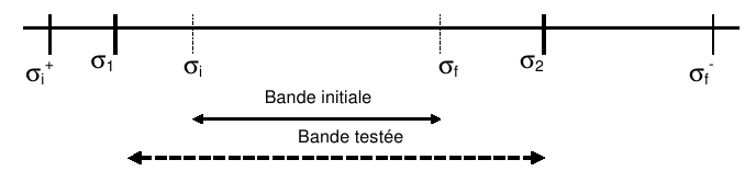
Figure 3.7-1. Eigenvalue counting by the Sturm test in GEP real symmetric.
By noting \({\sigma }_{i}^{+}\) and \({\sigma }_{f}^{-}\), respectively, the largest and the smallest eigenvalue not requested by the user and encompassing the initial band (cf. figure 3.7-1), we have the following algorithm for constructing the test band:
\(\begin{array}{c}\text{Si}{\sigma }_{i}^{+}\text{existe}(\text{resp}\text{.}{\sigma }_{f}^{-})\text{et si}\frac{\mid {\sigma }_{i}^{+}-{\sigma }_{i}\mid }{\mid {\sigma }_{i}\mid }<\text{PREC\_SHIFT}(\text{resp}\text{.}\frac{\mid {\sigma }_{f}^{-}-{\sigma }_{f}\mid }{\mid {\sigma }_{f}\mid })\\ \\ \text{alors}{\sigma }_{1}=\frac{{\sigma }_{i}^{+}+{\sigma }_{i}}{2}(\text{resp}\text{.}{\sigma }_{2}=\frac{{\sigma }_{f}^{-}+{\sigma }_{f}}{2}),\\ \text{Sinon}\\ {\sigma }_{1}={\sigma }_{i}(\text{1-}\text{sign}({\sigma }_{i})\text{PREC\_SHIFT})(\text{resp}\text{.}{\sigma }_{2}={\sigma }_{f}(\text{1+sign}({\sigma }_{f})\text{PREC\_SHIFT})),\\ \text{Fin si}\text{.}\end{array}\)
Algorithm 2. Construction of the test strip for the Sturm test.
This test strip construction sequence, via the calculated and unrequested modes, is only active for the Lanczos and Bathe & Wilson methods of CALC_MODES with OPTION =” BANDE “/ “CENTRE”/””/”PLUS_ *”/” TOUT”. With the Sorensen and QZ methods, only the requested modes are selected and therefore the limits of the test interval are determined by the second part of algorithm No. 2.
This algorithm is parameterized by the keyword PREC_SHIFT of the keyword factor VERI_MODE. The boxes below show the trace of error messages when these post-checks are triggered.
Retrospective verification of the modes
<E><ALGELINE5_15>
for concept MODE_B_1, mode number 5
Frequency 84.821272
has an error standard of 0.000102 greater than the accepted threshold 0.000001.
Retrospective verification of the modes
<E><ALGELINE5_23>
for the MODET concept,
in the meantime [28.987648 , 5071.142099]
theoretically there are 6 natural frequency (s)
and we calculated 5.
This problem can occur when there are multiple modes (structure with symmetries) or a high modal density.
Example 3. Impressions in the post-check message file.
The counting procedure can be deactivated via with the VERI_MODE/STURM keyword. Likewise, when at least one of the two post-verification steps (residue standard or counting procedure) is not respected, the sequence of events is controlled by STOP_ERREUR (if “OUI” the calculation stops, otherwise the error is just signalled by an alarm). Of course, we can highly recommend that you do not deactivate these “go-it-all” settings!
Notes:
When with the options “BANDE”, “CENTRE”, “”, “”, “PLUS_ “ or” TOUT “*we activate the improvement procedure (keyword*AMELIORATION =” OUI”), the Sturm test is not performed at the end of the first resolution step (by a subspace method). This is useless, since these modes are likely to be modified in the second stage, that of improvement (by a few iterations of the inverse power method). It is only after this step that all the checks are carried out: residue, Sturm test and belonging to the initial band (if*OPTION =” BANDE “*) . *
The Sturm test can also be activated with the options “ PROCHE “, “ “, “ SEPARE “ and “ AJUSTE “. It does*not quite the same function.* Indeed, these options are used to refine initial estimates of eigenvalues and to calculate the associated eigenvectors: the presence of “holes” in the calculated spectrum is a then*possible and lawful .* On the other hand, the other options (”BANDE” etc…) must calculate all the specified modes, not to mention some*r:*no holes in the spectrum is*then*tolerated. *
With “PROCHE”, “SEPARE” and “AJUSTE”, the emission of alarm or error messages therefore does not necessarily reveal a numerical problem but may be normal depending on the data set. So if one specifies FREQ =( 100.0,300.0) , that the option “ PROCHE “ refines these values in (99.0, 299.0) and that the spectrum of the mechanical problem normally also includes the value 200.0 , the Sturm test (if activated) will stop the calculation on an error message while this absence of the value 200.0 is normal. The user did not ask to refine it! With the initial settings FREQ =( 100.0, 200.0, 300.0) this alarm wouldn’t appear anymore.
In this context, the activation of the Sturm test should therefore be handled with care. Functionally, it is rather used to postpone verification tests when activating the keyword AMELIORATION at the end of a subspace method (cf. previous note) .
3.7.5. Display in the message file#
In the message file, information relating to the modes selected is mentioned. For example, in the most common case of a real symmetric GEP (real eigenmodes), we specify the modal solver used, the list of the \({f}_{i}\) frequencies used (FREQUENCE) and their error standard (NORME D” ERREUR, cf. algorithm No. 1).
CALCUL MODAL: METHODE GLOBALE FROM TYPE QR
ALGORITHME QZ_SIMPLE
NUMERO FREQUENCE (HZ) **** NORME D’ERREUR **
1 1.67638E+02 2.47457E-11
2 1.67638E+02 1.48888E-11
3 1.05060E+03 2.00110E-12
4 1.05060E+03 1.55900E-12
…
Example 4a. Impressions in the message file of the eigenvalues retained during GEP in real modes. Excerpt from the forma11a test case.
For a GEP with complex modes (not symmetric real or complex symmetric) [10] _ ), unlike QEP [Boi09], Code_Aster does not filter the conjugated eigenvalues of any complexes. It keeps all of them and displays them in ascending order of actual game. Thus, columns FREQUENCE and AMORTISSEMENT combine, respectively, \(\text{Re}({f}_{i})\) and \(\frac{\text{Im}({f}_{i})}{2\text{Re}({f}_{i})}\).
CALCUL MODAL: METHODE OF ITERATION SIMULTANEE
METHODE OF SORENSEN
NUMERO FREQUENCE (HZ) **** AMORTISSEMENT **** NORME D’ERREUR
1 5.93735E+02 5.00000E-03 2.73758E-15
2 9.45512E+02 5.00000E-03 1.64928E-15
3 3.51464E+03 5.00000E-03 2.14913E-15
…
Example 4b. Impressions in the message file of the eigenvalues retained during GEP in complex modes. Excerpt from the zzzz208a test case.
Now that the context of GEPs in Code_Aster has been outlined, we will focus on power-type methods and their implementation in the CALC_MODES operator with OPTION among [“PROCHE”, “AJUSTE”, “”, “SEPARE”].