1. Problem model and notations#
1.1. Equations#
An elastic solid, linked to a Cartesian coordinate system of \({ℝ}^{3}\), occupies, in its natural state and before deformation, a connected bounded open domain \(\Omega\) of \({ℝ}^{3}\) with a regular border \(\partial \Omega\) of an outgoing normal \(\overrightarrow{n}\). This outline is the union of two disjunct parts \({\Gamma }_{U}\) and \({\Gamma }_{F}\) such as \({\Gamma }_{U}\cup {\Gamma }_{F}=\partial \Omega\) and \({\Gamma }_{U}\cap {\Gamma }_{F}=\varnothing\).
Let \(\overrightarrow{u}(x)={u}_{1}(x)\overrightarrow{{e}_{1}}+{u}_{2}(x)\overrightarrow{{e}_{2}}+{u}_{3}(x)\overrightarrow{{e}_{3}}\) be the displacement of a point \(M\) from \(\Omega\) with coordinates \(x=({x}_{1},{x}_{2},{x}_{3})\). On the contour \({\Gamma }_{U}\), a movement \(\overrightarrow{u}(x)=\overrightarrow{0}\) is imposed and a surface force \(\overrightarrow{F}(x)\) is imposed on \({\Gamma }_{F}\). The solid is also subjected to a \(\overrightarrow{f}(x)\) volume force. The study is placed within the framework of linear elasticity and the hypothesis of small disturbances, without viscous damping.
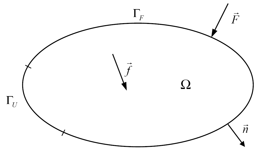
Figure 1.1-a : Undeformed configuration
In the following, we adopt the index notation for vectors and tensors, as well as the Einstein summation rule on repeated silent indices. For example, the following linear system:
: label: EQ-None
{begin {array} {c} {a} _ {11} {x} _ {1} _ {1} + {a} _ {12} {x} _ {2} = {b} _ {1}\ {a} _ {a} _ {21} {a} _ {a} _ {2} _ {1} _ {2} = {b} _ {2} _ {2} _ {2} _ {2} _ {2} _ {2} _ {2} _ {2} _ {2} _ {2} _ {2} _ {2} _ {2} _ {2} _ {2} _ {2} _ {2} _ {2} _ {2} _ {2} _ {2} _ {2} _ {2} _ {2}
can be written as:
: label: EQ-None
{a} _ {mathrm {ij}}} {x}} _ {j} = {b} _ {i}
The derivative of the \({i}^{\text{ème}}\) component of a \(\overrightarrow{v}\) vector with respect to the \({j}^{\text{ème}}\) component of space coordinates will be written as \({v}_{i,j}\).
The symmetric stress tensor \({\sigma }_{\mathrm{ij}}\) is linked to the linearized symmetric strain tensor \({\varepsilon }_{\mathrm{ij}}\) by the relationship:
: label: EQ-None
{sigma} _ {mathrm {ij}}} = {a} _ {mathrm {ijkl}} {varepsilon} _ {mathrm {ij}}} = {mathrm {ij}} = {a} _ {mathrm {ijkl}}
where \({a}_{\mathrm{ijkl}}\) is the elasticity coefficient tensor. It satisfies the relationships of:
symmetry: \({a}_{\mathrm{ijkh}}={a}_{\mathrm{jikh}}={a}_{\mathrm{ijhk}}={a}_{\mathrm{khij}}\);
positivity of the associated quadratic form: for any symmetric real tensor of the second order \({{\rm X}}_{\mathrm{ij}}\), \(\{\begin{array}{cc}\exists {\alpha }_{0}>\mathrm{0,}& \text{tel que}{{\rm X}}_{\mathrm{ij}}{a}_{\mathrm{ijkh}}(x){{\rm X}}_{\mathrm{kh}}\ge {\alpha }_{0}{{\rm X}}_{\mathrm{ij}}{{\rm X}}_{\mathrm{ij}}\\ \forall {{\rm X}}_{\mathrm{ij}}={{\rm X}}_{\mathrm{ji}},& \forall x\in \Omega \end{array}\).
The deformation tensor is linked to the displacement by the relationship:
: label: EQ-None
varepsilon (u) =frac {1} {2} (mathrm {grad} (u) + {mathrm {grad}}} ^ {T} {2} (u))
For a homogeneous and isotropic material, the law of behavior is Hooke’s law:
: label: EQ-None
sigma =lambdatext {tr} (varepsilon) I+2muvarepsilon
where \(\lambda\) and \(\mu\) are the Lamé coefficients.
The equilibrium equations, with the hypothesis of small disturbances, are written as:
: label: EQ-None
text {div}sigma +overrightarrow {f} =overrightarrow {0}
The boundary conditions defined above are written as:
: label: EQ-None
overrightarrow {u} (x) =overrightarrow {0}mathrm {on} {Gamma} _ {U}
: label: EQ-None
sigma (x)overrightarrow {n} (x) =overrightarrow {F} (x)mathrm {on} {Gamma} _ {F}
The set of equations is problem \(({\text{P}}_{1})\):
: label: EQ-None
{begin {array} {cccc} {sigma} _ {mathrm {ij}} _ {i} &text {=} & 0&text {in}text {in}Omega\ {sigma}} _ {sigma} _ {mathrm {sigma}} _ {mathrm {{sigma}} _ {mathrm {ijkh}} _ {mathrm {ijkh}} _ {varepsilon}} {varepsilon} _ {mathrm {kh}} &text {in}text {in}\ Omega\ {varepsilon} _ {mathrm {ij}} (u) &text {=} &frac {1} {1} {2} {2} (2)} ({u} {2}} (2}) (u) &text {1} {2} (in}) (u) &text {{=} & 0&text {on} {Gamma} _ {Gamma} _ {U}\ {sigma} _ {mathrm {ij}} {n} (x) &text {=} (x) &text {=} (x) &text {on} {gamma}} _ {f} (x) &text {on} {gamma}} _ {f} (x) &text {=}} & {F} & {F} & {F} & {F} & {F} & {F} & {F} & {F} & {F} & {F}} & {F} & {F}} & {F}
1.2. Variational formulation#
The space \(V\) is defined as the space of the admissible \(v\) functions, which are sufficiently regular, set to \(\Omega\) and have values in \({ℝ}^{3}\):
\(V=\left\{v\in {H}^{1}(\Omega )\text{et}v=0\text{sur}{\Gamma }_{U}\right\}\)
The standards related to it are as follows:
Standard \({L}^{2}\) |
\({\parallel v\parallel }_{{L}^{2}(\Omega )}^{2}=\underset{\Omega }{\int }v\cdot vd\Omega\) |
||
Standard \({H}^{1}\) |
\({\parallel v\parallel }_{{H}^{1}(O)}^{2}={\int }_{O}(v\cdot v+\nabla v:\nabla v)dO\) |
||
Semi-standard \({H}^{1}\) |
\({\mid v\mid }_{{H}^{1}(O)}^{2}={\int }_{O}\nabla v:\nabla vdO\) |
||
Energy Standard |
\({\parallel v\parallel }_{e}^{2}={\int }_{O}\sigma (v):\epsilon (v)dO\) |
The equilibrium equation is multiplied by a sufficiently regular function \(v\in V\) and then integrated into the domain \(\Omega\):
: label: EQ-None
0= {int} _ {omega} {sigma}} _ {mathrm {ij}, j} {v} _ {i} domega + {int} _ {omega} {f} _ {i} {f} _ {i} {f} _ {i} domega
: label: EQ-None
0= {int} _ {omega} {({sigma} _ {sigma} _ {mathrm {ij}}} {v} _ {i})} _ {, j} dOmega - {int} _ {omega} {omega} {omega} {sigma} {sigma} _ {sigma} _ {sigma} _ {sigma} _ {sigma} _ {sigma} _ {sigma} _ {omega} {sigma} _ {sigma} _ {sigma} _ {sigma} _ {sigma} _ {sigma} _ {sigma} _ {sigma} _ {sigma} _ {sigma} _ {sigma} _ {sigma} _ {sigma} _ {sigma} _ {sigma} _ {sigma} _ i} {v} _ {i} dOmega
Applying Green’s formula gives:
: label: EQ-None
{int} _ {Omega} {({sigma}} _ {mathrm {ij}}} {v} _ {i})} _ {, j} dOmega = {int} _ {partialOmega} _ {partialOmega}} {partialOmega} {partialOmega} {omega} {sigma} _ {sigma}} {sigma} _ {i} dGamma
The symmetry properties of the stress tensor involve:
: label: EQ-None
{sigma} _ {mathrm {ij}}} {v}} {v} _ {i, j} = {sigma} _ {mathrm {ij}} {varepsilon}} _ {mathrm {ij}} (v)
This allows you to write:
: label: EQ-None
{int} _ {partialOmega} {sigma} {sigma} _ {mathrm {ij}}} {n} _ {j} {v} _ {i}mathrm {dGamma} - {int} - {int} _ {omega} {omega} {a}} _ {mathrm {ijkh}}} {mathrm {}} (u) {omega} {a} _ {mathrm {ijkh}} {mathrm {}} (u) {omega} {a}} _ {mathrm {ijkh}} varepsilon} _ {mathrm {ij}} (v) domega + {int} _ {omega} {f} _ {i} {v} _ {i} domega =0
The first term on the second member is null on \({\Gamma }_{U}\) and it’s left:
: label: EQ-None
{int} _ {{Gamma} _ {F}} {F}} {F}} {F}} {F} _ {i}mathrm {dGamma} - {omega} {a} _ {mathrm {ijkh}} {mathrm {ijkh}}} {varepsilon}} _ {mathrm {ijkh}}} {mathrm {ijkh}}} (u) {varepsilon} _ {mathrm {ijkh}} _ {mathrm {ijkh}}} thrm {ij}} (v) dOmega + {int} _ {omega} {f} _ {i} {v} _ {i} domega =0
The variational formulation of problem \(({\text{P}}_{1})\) reads [bib1]:
: label: EQ-None
{begin {array} {cc}text {Find} uin Vtext {such as} &\ a (u, v) =l (v) &forall vin Vin Vend {array}
with:
: label: EQ-None
a (u, v) = {int} _ {omega} {a} {a} _ {mathrm {ijkh}} {varepsilon}} _ {mathrm {kh}} (u) {varepsilon}} (u) {varepsilon}} (u) {varepsilon}} (u) {varepsilon}} (u) {varepsilon}} (u) {varepsilon}} (u) {varepsilon}} (u) {varepsilon}} (u)
: label: EQ-None
l (v) = {int} _ {{Gamma} _ {F}} {F}} {F} {F}} {F} _ {i} dGamma + {int} _ {Omega} {f} {f} _ {i} {f} _ {i} dOmega
1.3. Finite element discretization#
Let \({\Omega }^{h}\) be a partition of \(\Omega\) in \(N\) elements. A finite element space \({V}^{h}\subset V\) is constructed from continuous functions, piecewise polynomial, and of degree \({p}_{E}\) on each element \(E\). Discretizing problem \(({\text{P}}_{1})\) by Galerkin’s method provides problem \(({\text{P}}_{h})\) [bib1]:
: label: EQ-None
{begin {array} {cc}text {Find} {u} {u} ^ {h}in {V} ^ {h}text {such as} &\ a ({u} ^ {h}, {v} ^ {h}, {v} ^ {h}) =l ({v} ^ {h}) =l ({v} ^ {h}) =l ({v} ^ {h}) =l ({v} ^ {h}) =l ({v} ^ {h}) =l ({v} ^ {h}) =l ({v} ^ {h}) =l ({v} ^ {h}) =l ({v} ^ {h}) =l ({v} ^ {h}) =l ({v} ^ {h}
1.4. Discretization error#
The numerical error \(e\) of the finite element approximation \({u}^{h}\) is defined by:
: label: EQ-None
e=u- {u} ^ {h}
As \(u\) and \({u}^{h}\) are elements of \(V\) then \(e\in V\). The error satisfies the residue equation obtained by replacing \(u\) with \({u}^{h}+e\) in the variational formulation of the problem \(({\text{P}}_{h})\):
: label: EQ-None
begin {array} {cc} a (e, v) =l (v) =l (v) -a ({u} ^ {h}, v) = {R} _ {h} ^ {u} (v) &forall vin Vend {array}
As the bilinear form is positive, residue \({R}_{h}^{u}\) is a linear form bounded on \(V\) that belongs to its dual \({V}^{\text{'}}\). The residue standard is such that:
: label: EQ-None
{parallel {R} _ {h} ^ {u}parallel} _ {{V}} _ {{V} ^ {text {“}}} =underset {vin Vsetminusleft{0right} {0right}}} {text {u}}}} {text {u}left{0right}}}} {text {u}}}} {text {u}left{0right}}}} {text {u}}}} {text {u}left{0right}}}} {text {u}}}} {text {u}left{0right}}}} {text {u}}}} {text {u}}}}
The residue measures the non-verification of certain properties of the equations of the problem and characterizes the balance faults and therefore the discretization error. It is easy to deduce a new property from the equation. Function \({v}^{h}\) is used as a test function:
: label: EQ-None
begin {array} {cc} {R} _ {h} _ {h} _ {h} _ {h} _ {h} _ {h} _ {r} _ {r} _ {h}, {v} ^ {h}, {v} ^ {h}) &forall {v} ^ {h}) &forall {v} ^ {h}) &forall {v} ^ {h}) &forall {v} ^ {h}) &forall {v} ^ {h}) &forall {v} ^ {h}) &forall {v} ^ {h}) &forall {v} ^ {h})
Then using the discretized form of the variational formulation, the orthogonality property or Galerkin property is obtained:
: label: EQ-None
begin {array} {cc} a (e, {v} ^ {h}) = {R} _ {h} ^ {u} ({v} ^ {h}) =0&forall {v} ^ {h} ^ {h}in {V} ^ {h}end {array} ^ {h}) =0&forall {v} ^ {h} ^ {h}) =0&forall {v} ^ {h} ^ {h}) =0&forall {v} ^ {h} ^ {h}) =0&forall
The equation indicates that the error is the solution of an elasticity problem in which the force load is the equilibrium residue. This problem is as complicated to solve and expensive as the original problem. Thus, instead of determining the error itself, estimates will be sought.
1.5. A priory error estimation#
As its name suggests, a priori estimation is done before finite element calculation because it does not involve the finite element approximation \({u}^{h}\). Thus, functional analysis and numerical analysis make it possible, in many cases and under certain assumptions of regularity, to obtain estimation results a priori; that is to say the prediction of the asymptotic convergence rate of the finite element error. For more details, the books by Ciarlet [bib1] or Strang and Fix [bib2] can be consulted.
A \(\tilde{\eta }(h,d,u)\) function is an a priori error estimate if:
where \(\parallel \cdot \parallel\) is a standard for travel fields, \(h\) is the size of elements, \(d\) is a data set of the problem, and \(u\) is the exact solution.
The convergence of the finite element method used can be obtained if:
and the convergence rate, if there is a real \(q>0\) such as:
a priori error estimators do not make it possible to quantify errors in the finite elements solution because they involve the exact solution, which is generally not known. On the other hand, these estimates are only valid in the asymptotic regime, a regime that is difficult to achieve for 3D calculations. For formulations using isoparametric elements [bib2], in the case of a regular solution and for the error energy standard, \(q=p\), where \(p\) is the degree of interpolation of the finite elements. On the other hand, in the case of a singular solution, \(q=\text{min}(p,\alpha )\) where \(\alpha\) is the order of the singularity of the solution of the problem (for a crack, for example, \(\alpha =\frac{1}{2}\)).