3. Local error#
3.1. Pollution error#
3.1.1. Definition of pollution error#
To define the pollution error, we will provide a pragmatic definition by trying to understand what its behavior and therefore its influence may be during an adaptive process. To do this, we will study the convergence of the error into the energy norm in different situations:
Convergence of the global error for a uniform global refinement;
Convergence of the error in the area of interest for global refinement;
Convergence of the global error for local refinement;
Convergence of the error in the area of interest for local refinement.
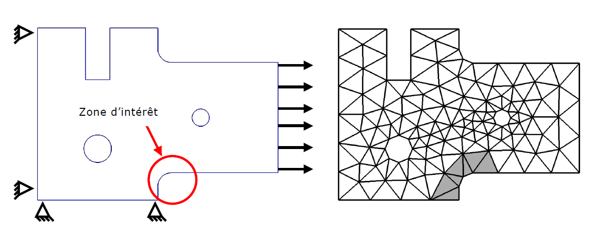
Figure 3.1.1-a : Geometry and mesh (192 elements) .
The problem to be solved is the problem whose geometry and mesh are given by the figure. The force imposed is unitary, the Young’s modulus is equal to \(E=1.0\) Pa and the Poisson’s ratio is equal to \(\nu =0.3\). Finally, the modeling used is a modeling using plane constraints. A series of finite element approximations will be determined on a succession of linear meshes obtained by uniform refinement of the structure or by uniform refinement of the zone of interest \(\omega\). The energy norm error is then calculated (therefore without estimation) from a solution obtained on a very fine mesh (overkill solution) which will be our reference solution. Finally, the absolute error is normalized by the energy standard of the solution on the structure or on the zone of interest as the case may be. The results are shown in the figure.
For global refinement, the global error converges « a bit slower » than \(p=1\); by dividing the mesh size by 10, the error is not divided by 10 (even when dividing the size by 16 the error is not divided by 10) (square markers). However, this convergence speed is only achieved asymptotically. It should be noted that the curve represented seems to approach the theoretical convergence starting from the last segment (for mesh sizes between 1/8 and 1/16). It is therefore only the first part of a convergence curve that is drawn, when convergence in \(p=1\) has not yet been reached (pre-asymptotic regime).
When only the area of interest is refined, the solution is not improved in the rest of the structure. The overall error remains virtually unchanged (round markers). This indicates that the error in the area of interest contributes very little to the overall error.
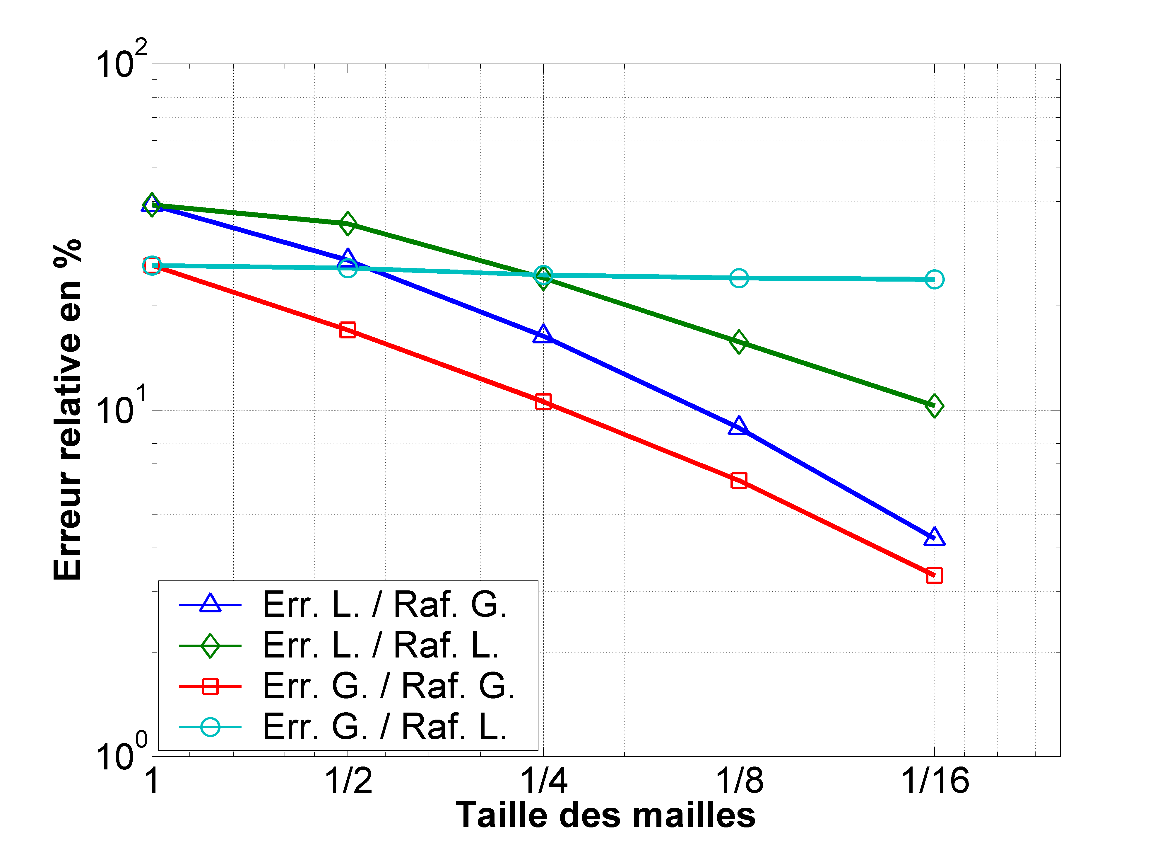
Figure 3.1.1-b : Highlighting the pollution error: convergence of the error.
On the other hand, by studying the curves relating to the error in the zone of interest, it is visible that in order to significantly improve the solution in this zone it is not sufficient to refine this zone alone. In fact, the two curves (diamond markers and triangular markers) show a decrease in the local error but that obtained by local refinement shows a slower decrease: the two curves differ. It therefore seems that the error in the rest of the structure also has an influence on the quality of the solution in the area of interest. This means that the sum of the local contributions of the global estimators on subdomain \(\omega\) does not exactly represent the local error. It therefore seems that the true local error is composed of two parts: a local component and a complementary component from the rest of the structure. The consequence of this is that by refining only the area of interest, the error in the rest of the structure does not decrease (i.e. the complementary component remains constant). We can then imagine that the curve representing the local error with a local refinement (diamond markers) converges to a non-zero value if the refinement is continued: this non-zero value will represent the complementary component (the local component tending towards zero). The value of the complementary component is then called « pollution error ».
A more formal definition can be given. The pollution error was introduced by Babuška et al. [bib16], [bib17], [bib18]. They assume that the discretization error in a sub-domain \(\omega\) of the structure is composed of:
a local error on \(\omega\), ignoring the rest of the structure;
from a pollution or transport error, resulting from discretization in the rest of the structure.
The fundamental relationship between the global error \(e\) and the \({\Phi }_{E}\) solution of the local error problem (solution resulting from the Equilibrated Residual Method for example) is recalled:
: label: EQ-None
begin {array} {cc} a (e, v) =sum _ {EinOmega} {a} _ {E} ({Phi} _ {E}, v) &forall vin Vin Vend {array}
A local error \({e}_{\omega }^{\text{loc}}\) on a \(\omega\) subdomain can be defined by:
: label: EQ-None
begin {array} {cc} a ({e} _ {omega}} ^ {text {loc}}, v) =sum _ {Esubsetomega} {a} _ {E} _ {E} ({varphi}} _ {omega}} _ {omega}} ^ {omega} ^ {text {loc}}, v) =sum _ {E}omega} {a} _ {E} _ {E} ({varphi}} _ {E}} _ {E}} ({varphi}} _ {omega} _ {omega} _ {omega} _
As the local error indicator function \({\varphi }_{E}\) only depends on the local residuals of the finite element approximation evaluated on the element patch \(E\text{*}\), the local error \({e}^{\text{loc}}\) only depends on the local residuals on the patch \(\tilde{\omega }\), which consists of the elements of \(\omega\) and the neighboring elements. The complementary component of the true error is pollution error \({e}_{\omega }^{\text{pol}}\):
: label: EQ-None
begin {array} {cc} a ({e} _ {omega} _ {omega}} ^ {text {pol}}, v) =sum _ {Enotsubsetomega} {a} {a} _ {E}} ({E}} _ {E}, v) &forall vin Vend {array}
This part of the true error comes from residues located outside the subdomain and is carried to the subdomain, thus affecting accuracy. The error \({e}_{\omega }\) in a \(\omega\) sub-domain is therefore the sum of the two components defined above:
: label: EQ-None
{e} _ {omega} = {e} _ {omega} ^ {text {loc}} + {e} _ {omega} ^ {text {pol}} ^ {text {pol}}
In view of the figure and the previous definition, it becomes obvious that controlling the pollution error is essential. In fact, outside the area of interest, when the mesh is coarse, it can be a major source of pollution error. As a result, local refinement on a subdomain must be counterbalanced by adequate refinement outside the subdomain in order to control the pollution error. We will see in the following that the estimators of error in quantity of interest make it possible to ensure this balance between local refinement and refinement outside the subdomain.
3.1.2. Estimation of the pollution error#
To estimate the pollution error, various methods have been proposed. The method proposed by Babuška (Babuška et al., 1995) is linked to Green’s functions that describe the interaction between different points in the domain. The pollution error is estimated with the error in approximating the Green function associated with certain points. Another method was used by Huerta and Díez (Huerta & Díez, 2000) and consists of finding an approximation of \({e}_{\omega }^{\text{pol}}\) by solving the problem that defines this error. Other works can also be cited (Ainsworth, 1999), (Oden & Feng, 1996). Since the industrial value of evaluating this error is limited, we will not further develop these estimation methods. The numerous works on the calculation of error limits make it useless to estimate the pollution error because it is included in the limits. In addition, for the estimation of a local error, as we have already indicated, the estimators in terms of quantity of interest make it possible to get rid of the pollution error thanks to the dual problem.
3.2. Error in quantity of interest#
3.2.1. Quantities of interest#
Energy standard error estimates are too abstract to provide users of calculation codes with sufficient information on the various aspects of the solution sought. It is then more useful to estimate an error in terms of quantities of interest; quantities that have a physical meaning (an average of movements in a sub-region of the physical domain or an average of constraints on an interface or even, in the case of vibrations, one of the natural frequencies). Mathematically, they are characterized by linear or non-linear functionals in the space of functions to which the solutions belong.
Several examples are given: the average of a component of the displacement on a domain \(\omega\):
: label: EQ-None
Q (v) =frac {1} {midomegamid} {omegamid} {int} _ {omega} {v} _ {x} domega
the average of a component of the stress tensor on a domain \(\omega\):
: label: EQ-None
Q (v) =frac {1} {midomegamid} {omegamid} {int} _ {omega} {sigma} _ {mathrm {xx}} domega
We then try to calculate the quantity \({\varepsilon }^{Q}\) which can be expressed in the following form:
: label: EQ-None
{varepsilon} ^ {Q} =Q (u) -Q ({u} ^ {h})
In the case where \(Q\) is linear, the following equality is true:
: label: EQ-None
{varepsilon} ^ {Q} =Q (u- {u} ^ {h}) =Q (e)
In the following, only the case of linear functionals will be considered because this corresponds to the framework of the simplified approach presented below. In general, the treatment used for non-linear quantities (such as the Von Mises stress or the \(J\) integral in fracture mechanics) is linearization [bib19] and [bib20].
3.2.2. Dual problem and fundamental relationship#
The error in quantity of interest can be estimated by using duality properties of the operators involved in the weak formulation of the reference problem. From a mechanical point of view, this corresponds to the existence of a dual problem solution function, called an influence function, representing the influence of the efforts of the reference problem on the total energy. The influence function is then used as a weighting of the equilibrium residuals of the reference problem.
A simplified approach is presented, in that the framework is limited to linear elasticity and linear quantities of interest. This means that \(Q(\cdot )\) is a linear form and \(a(\cdot ,\cdot )\) is a bilinear form. This approach makes it possible to better understand the need to use the error on the influence function and not only the influence function.
The relationship between the error in quantity of interest and the residue can be expressed by the introduction of an unknown function \(\omega\), called an influence function:
: label: EQ-None
Q (e) =omega ({R} _ {h} ^ {u})
In addition, we show in [bib21] that the previous relationship becomes:
: label: EQ-None
Q (e) = {R} _ {h} ^ {u} (omega)
Combining the previous relationship with the residue equation:
: label: EQ-None
a (e, v) = {R} _ {h} ^ {u} (v)
a relationship between the error on the reference problem, the influence function and the error in quantity of interest is obtained:
: label: EQ-None
a (e,omega) =Q (e)
This equality is necessarily verified when \(\omega \in V\) is the solution of the following problem:
: label: EQ-None
{begin {array} {cc}text {Find}text {Find}omegain Vin Vtext {tel}text {que} &\ a (v,omega) =Q (v) &forall vin Vin Vend {array}
This problem is called a dual or adjunct problem. Note that if \(\omega\) could be calculated exactly, then \(Q(u)\) could be determined directly from the problem data because:
: label: EQ-None
Q (u) =a (u,omega) =l (omega)
But unfortunately, it is as difficult to determine the \(\omega\) influence function as it is to determine \(u\) in the primal problem. This is why a finite element approximation \({\omega }^{h}\in {V}^{h}\) of \(\omega\) that satisfies
: label: EQ-None
begin {array} {cc} a ({v} ^ {h}, {omega} ^ {h}) =Q ({v} ^ {h}) &forall {v} ^ {h}in {V} ^ {h}in {V} ^ {h}end {array}
is introduced. We also note that by substituting \(e\) to \({v}^{h}\) in the dual problem, we obtain:
: label: EQ-None
Q (e) =a (e,omega)
Replacing \(\omega\) by \({\omega }^{h}\) in the previous relationship is not enough to get an estimate of \(Q(e)\) because \(a(e,{\omega }^{h})=0\) (orthogonality property). This is why it is necessary to evaluate the error on the influence function noted \(\varepsilon =\omega -{\omega }^{h}\). By introducing this error into the previous relationship, a representation of the error is obtained:
: label: EQ-None
Q (e) =a (e,varepsilon)
In the case of nonlinear problems and/or nonlinear quantities of interest, the above does not apply. In this case, the primal problem is written as:
: label: EQ-None
{begin {array} {cc}text {Find} uin Vtext {such as} &\ A (u; v) =L (v) &forall vin Vin Vend {array}
where \(A(\cdot ;\cdot )\) is a semi-linear form such that the arguments following the semicolon are linear and \(L(\cdot )\) is a linear form that is continuous over \(V\).
The approach consists in considering the primal problem as a problem of minimization under constraint [bib19], [bib20]:
: label: EQ-None
{begin {array} {c}mathrm {Find} uin Vmathrm {tel}mathrm {que}\ Q (u) =underset {zin S} {text {inf}} {text {inf}}} Q (z}}} Q (z}}} Q (z)}} Q (z)}} Q (z)}} Q (z)} Q (z)} Q (z)} Q (z)} Q (z)} Q (z)} Q (z)} Q (z)} Q (z)} Q (z)} Q (z)} Q (z)} Q (z)} Q (z)} Q (z)} Q (z)} Q (z)} Q (z)} Q (z)} forall vinin Vright}end {array}
To solve the minimization problem, the \((u,\omega )\in V\times V\) couple is sought such that it satisfies the primal problem and the dual problem:
: label: EQ-None
{begin {array} {cc} A (u;tilde {v}) =L (tilde {v}) &foralltilde {v}in V\ {A} ^ {text {”} ^ {text {“}} ^ {text {“}} ^ {text {v}}in Vend {array}} (u; v) ^ {text {“}} ^ {text {“}} ^ {text {“}} ^ {text {“}} ^ {text {“}} ^ {text {“}} ^ {text {“}} ^ {text {“}} ^ {text {“}} ^ {text {“}} ^ {text {“}} ^ {text {“}} ^
Finally, the relationship between the error in quantity of interest \({\varepsilon }^{Q}\) and the residue is given by:
: label: EQ-None
{epsilon} ^ {Q} =Q (u) -Q ({u} -Q ({u} ^ {h}) =R ({u} ^ {h};omega) +mathrm {Delta A} +mathrm {Delta Q}
where \(\Delta A\) and \(\Delta Q\) involve the second and third derivatives of \(A\) and \(Q\).
3.2.3. Estimation of the error in quantity of interest#
Based on the fundamental relationship, various techniques have been developed in order to estimate the error in terms of quantity of interest.
The simplest and most direct technique is to use global estimators as an energy norm. By applying the Cauchy-Schwartz theorem, a relationship between the error in quantity of interest and the energy norms of the errors on the primal problem and the dual problem can be found [bib22]:
: label: EQ-None
mid Q (e)midle {parallel eparallel} _ {e} {parallelvarepsilonparallel} _ {e}
This expression thus allows us to easily estimate the error in terms of quantity of interest using any energy standard error estimator, without additional development in a calculation code that has global estimators. Although this estimate is the simplest, it is also the crudest: it does not take into account the local interactions between the primal error and the dual error (schematically this means that an error in displacement does not translate into an error in quantity of interest). This can lead to severe overestimates of the error in terms of quantity of interest.
A slightly different approach, called*Dual Weighted Residual* (DWR) [bib19], is to consider the exact expression of the error in terms of quantity of interest:
: label: EQ-None
Q (e) =a (e,omega - {omega} ^ {h}) = {R} _ {h} ^ {u} (omega - {omega} ^ {h})
The dual problem is solved using a high order approximation method. Another method, less expensive, consists in using high-order interpolation functions defined on elementary patches in the domain. This approach leads to a guaranteed upper bound of error.
An « exact bounds » approach (exact bounds approach) [bib23] uses the properties of the estimate based on dual analysis. Thus, thanks to a displacement formulation of the finite element method, a lower bound of the exact deformation energy is obtained; thanks to a stress formulation, an upper bound of the exact complementary energy is obtained. From a practical point of view, this method is very expensive since it involves solving twice the primal problem and the dual problem.
Other methods exist to estimate the error in terms of quantity of interest but from an industrial point of view, only the approach using global estimators in energy standards seems to be convincing. It does not require additional development to access an indication of the error and it is also much less expensive.
3.2.4. Boundaries of error#
3.2.4.1. A new expression for error#
Although very simple to obtain, the relationship produces a significant overestimation of the error. Various techniques have been proposed to remedy this problem. Prudhomme and Oden use the parallelogram relationship for problems with symmetric bilinear shapes giving access to an upper bound and a lower bound of the error [bib24], [bib21].
If \(e\) and \(\varepsilon\) are the errors of the finite element approximations, respectively the solutions of the primal and dual problems then:
: label: EQ-None
Q (e) =a (e,varepsilon) =frac {1} {4} {parallel e+varepsilonparallel} _ {e} ^ {2} -frac {1} {1} {4} {frac {1} {4} {4} {parallel e-varepsilonparallel} _ {e} ^ {2} -frac {1} {4} {4} {4} {parallel e-varepsilonparallel} _ {e} ^ {2}
We introduced the scalar factor \(s\in R\)
: label: EQ-None
Q (e) =a (e,varepsilon) =frac {1} {1} {4} {parallel se+ {s} ^ {-1}varepsilonparallel} _ {e} ^ {2} -frac {1} {2} -frac {1} {2} -frac {1} {1} -frac {1} {2} -frac {1} {1} {2} -frac {1} {1} {2} -frac {1} {1} {2} -frac {1} {1} {2} -frac {1} {1} {2} -frac {1} {1} {2}
The scalar \(s\) is chosen so that the quantities \({\parallel se\parallel }_{e}\) and \({\parallel {s}^{-1}\varepsilon \parallel }_{e}\) have the same amplitude, which implies choosing \(s=\sqrt{{\parallel \varepsilon \parallel }_{e}/{\parallel e\parallel }_{e}}\).
Indeed \(e\) and \(\varepsilon\) can be of very different orders of magnitude. The scalar \(s\) aims to « standardize » the two terms, in order to avoid making a difference between two very similar terms because this can induce a significant numerical error.
Formally, any existing error estimator can be used to evaluate the energy standards of the parallelogram relationship; the more « fair » this estimate is, the better the quality of the error estimator in terms of quantity of interest will be.
3.2.4.2. Construction of bollards#
The global estimators \({\eta }_{\mathrm{inf}}^{\text{+}}\), \({\eta }_{\text{sup}}^{\text{+}}\), \({\eta }_{\mathrm{inf}}^{\text{-}}\), and \({\eta }_{\text{sup}}^{\text{-}}\) are defined as:
: label: EQ-None
{eta} _ {text {inf}}} ^ {text {+}}}le {parallel se+ {s} ^ {-1}varepsilonparallel} _ {e}le {eta}}le {eta}} _ {text {+}} _ {text {+}}
: label: EQ-None
{eta} _ {text {inf}}} ^ {text {-}}}le {parallel se- {s} ^ {-1}varepsilonparallel} _ {e}le {eta}}le {eta}} _ {text {-}} _ {text {-}}
By rewriting the two previous inequalities as follows:
: label: EQ-None
frac {1} {4} {({eta}} _ {mathrm {inf}}} ^ {text {+}})} ^ {2}lefrac {1} {4} {parallel se+ {s} + {s} {s} {s} ^ {-1}}varepsilon {-1} {-1}} {eta} _ {text {sup}}} ^ {text {+}})} ^ {2}
: label: EQ-None
frac {1} {4} {({eta}} _ {mathrm {inf}}} ^ {text {-}})} ^ {2}lefrac {1} {4} {parallel se- {s} {s} _ {s} ^ {-1}}varepsilon {-1} {-1}} {eta} _ {text {sup}}} ^ {text {-}})} ^ {2}
and adding them up:
: label: EQ-None
frac {1} {4} {({eta}} _ {mathrm {inf}}} ^ {text {+}})} ^ {2} -frac {1} {4} {({eta}} _ {eta} _ {eta} _ {text {sup}} _ {text {sup}}}} ^ {text {-}})} ^ {2}thefrac {1} {4} {{4} {parallel se+ {s}} {parallel se+ {s} ^ {-1}varepsilonparallel} _ {e} ^ {2} _ {e} ^ {2} -frac {1} {4} {parallel se- {s} ^ {-1}varepsilonparallel} _ {e}} _ {e}} _ {text {parallelparallelparallel}} _ {text {+}} ^ {text {+}})} ^ {2} -frac {1} {4} {4} {({eta}} _ {text {inf}}} ^ {text {-}})})} ^ {2}
a framework for the error in terms of quantity of interest is obtained.
Then the terminals \({\eta }_{\text{inf}}^{Q}\), \({\eta }_{\text{sup}}^{Q}\) are introduced such as:
: label: EQ-None
{eta} _ {text {inf}}} ^ {Q}} ^ {Q} =frac {1} {1} {4} {({eta}} _ {text {inf}}} ^ {}})} ^ {2}} -frac {1} {Q} =frac {1} {Q}} =frac {1} {Q}} =frac {1} {Q}} =frac {1} {4} {4} {({eta}} _ {text {inf}}} ^ {-}})} ^ {2} -frac {1} {Q} = =frac {1} {Q}} =frac {1} {Q} = {1} {Q} =
: label: EQ-None
{eta} _ {text {sup}}} ^ {Q}} ^ {Q} =frac {1} {4} {({eta} _ {text {sup}}} ^ {}})} ^ {2}} -frac {1} {Q} =frac {1} {Q}} =frac {1} {Q}} =frac {1} {Q}} =frac {1} {4} {4} {({eta}} _ {text {sup}}} ^ {-}})} ^ {2} -frac {1} {Q} = =frac {1} {Q}} =frac {1} {Q}} =frac {1} {Q} {
The interest quantity error \(Q(e)\) is bounded by \({\eta }_{\text{inf}}^{Q}\) and \({\eta }_{\text{sup}}^{Q}\):
: label: EQ-None
{eta} _ {text {inf}}} ^ {Q}le Q (e)le {eta} _ {text {sup}}} ^ {Q}
It is also possible to use the estimates \({\eta }_{\text{eei}}^{Q}\) and \({\eta }_{\mathrm{ees}}^{Q}\) defined such as:
: label: EQ-None
{eta} _ {text {eei}}} ^ {Q}} ^ {Q} =frac {1} {1} {4} {({eta}} _ {text {inf}}} ^ {}})} ^ {2}} -frac {1} {Q} =frac {1} {Q}} =frac {1} {Q}} =frac {1} {Q} {4} {({eta}} _ {text {inf}}} ^ {-}})} ^ {2} -frac {1} {Q}} =frac {1} {Q}} =frac {1} {Q}} =frac {1} {Q}} =frac {1} {
: label: EQ-None
{eta} _ {text {ees}}} ^ {Q}} ^ {Q} =frac {1} {4} {({eta} _ {text {sup}}} ^ {}})} ^ {2}} -frac {1} {Q} =frac {1} {Q}} =frac {1} {Q}} =frac {1} {Q}} =frac {1} {4} {4} {({eta}} _ {text {sup}}} ^ {-}})} ^ {2} -frac {1} {Q} = =frac {1} {Q}} =frac {1} {Q}} =frac {1} {Q} {
as an estimate of the error in quantity of interest \(Q(e)\).
Finally, a final estimate can be obtained, by using the limits \({\eta }_{\text{inf}}^{Q}\) and \({\eta }_{\text{sup}}^{Q}\) or the estimates \({\eta }_{\mathrm{eei}}^{Q}\) and \({\eta }_{\mathrm{ees}}^{Q}\), noted \({\eta }_{\mathrm{moy}}^{Q}\):
: label: EQ-None
begin {array} {ccc} {eta}} _ {mathrm {moy}}} ^ {Q} & =&frac {1} {2} ({eta} _ {mathrm {eei}}}} ^ {eei}}}} ^ {2}} ^ {Q})\ & =&frac {1} {2}}} ^ {Q})\ & =&frac {1} {2} ({eta} _ {text {inf}}} ^ {Q} + {eta} + {eta} _ {text {sup}} ^ {Q})\ & =&frac {1} {8} ({({eta}} _ {eta} _ _ {eta} _ {eta} _ {eta} _ {eta} _ {eta} _ {eta} _ {eta} _ {eta} _ {eta} _ {eta} _ {eta} _ {eta} _ {eta} _ {eta} _ {eta} _ {eta} _ {eta} _ {eta} _ {eta} _ {eta} _ {eta} _ {eta} _ {eta} _ {eta} _ {text {+}})} ^ {2}) -frac {1} {8}) -frac {1} {8}} ({({eta}})} ^ {2})} ^ {2} + {({eta} + {eta} _ {eta} _ {text {sup}}} {text {-}} _ {text {-}}} ^ {2})} ^ {2})end {array} + {eta} _ {eta} _ {text {sup}}} ^ {2})end {array} + {eta} _ {eta} {8}} ({eta}} {8}} ({eta}}) {
The following figure summarizes the various possible combinations of the energy norm error estimate to obtain an estimate or bounds of the error in quantity of interest. This shows that if we have bounds for an energy norm estimator then we have bounds for the error in terms of quantity of interest.
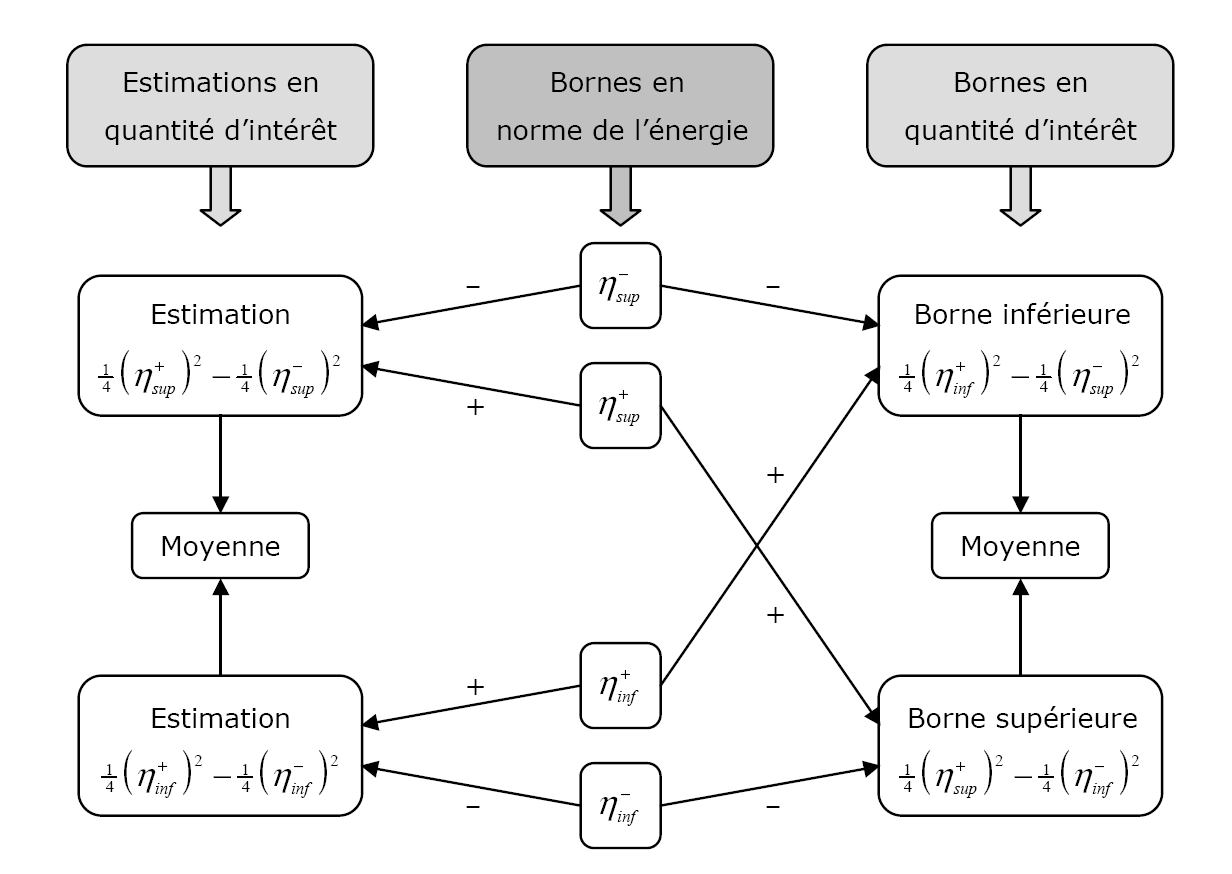
Figure 3.2.4.2-a : Estimates and limits of the error in quantity of interest (Prudhomme et al., 2003).
3.2.4.3. Estimates of the limits of error#
In the previous chapter, it was shown that global error limits were accessible using implicit residue estimators. The main lines are given here to obtain limits of the error in quantity of interest using the implicit estimators. It should be noted that this is only an example and that other estimation methods can provide bounds for the error in terms of quantity of interest.
In order to obtain the upper limits defined above, the functions \({\psi }_{E}^{u}\) and \({\psi }_{E}^{\omega }\), corresponding respectively to the errors \(e\) and \(\varepsilon\), are calculated by introducing the local problems relating to the primal and dual problems. The following estimates are then obtained:
: label: EQ-None
{eta} _ {text {sup}}} ^ {text {+}}} = {parallel s {psi} _ {E} ^ {u} + {s} ^ {-1} {-1} {psi} {psi} {psi} {psi} _ {psi} _ {e} _ {e}
For the estimation of the lower limits, it is necessary to proceed in the same way as for the estimation of the upper limits by constructing continuous functions at the interfaces from \({\psi }_{E}^{u}\) and \({\psi }_{E}^{\omega }\):
: label: EQ-None
{eta} _ {text {inf}}} ^ {text {+}} ^ {text {+}}} =frac {0,0 (s} _ {-1} {R} _ {h} _ {h} ^ {omega}) ^ {omega})) (s {chi} ^ {omega}) (s {chi}} {omega} _ {h}} {omega} _ {h}} _ {h} _ {h}} _ {h} _ {h} _ {h} _ {h} _ {h} _ {h} _ {h} _ {h} _ {h} _ {h}} _ {h} _ {h} _ {h} _ {h} _ {h}} _ {h} _ {h} _ {h} _ {h} {chi} _ {E} ^ {u} + {s} ^ {-1} {chi} _ {E} ^ {omega}parallel} _ {e}}