2. Development of the method#
2.1. Principles of the method#
The proposed method is based on the simple hypothesis that the response of the floor without Floor-Material Interaction (IPM) can be assimilated to the response of a 1D oscillator with frequency \({f}_{1}\), mass \({m}_{1}+{m}_{2}\) and damping \({\xi }_{1}\) (see Figure 2), where we have defined \({m}_{1}\) as the mass of the floor and \({m}_{2}\) the mass of the equipment (see Figure 2), where we have defined as the mass of the floor and the mass of the equipment.
It is the flexure mode of the floor panels that is taken into account by the one-dimensional modeling of the floor. We also consider that the modal mass mobilized by the flexure mode is the total mass of the floor, which is a conservative hypothesis. The answer of the floor without IPM is the same as considering that the mass equipment \({m}_{2}\) is rigidly connected to the floor.
For its part, the equipment is characterized by a set of 1D oscillators of varying frequencies and masses. In fact, we assume that heavy equipment placed on the floor has several natural frequencies in the vertical direction. The modal characteristics of the equipment (frequencies and participative masses) are to be determined prior to the calculation by the user. This data can be found in qualification notes or sizing notes. A finite element calculation can also provide this type of information. Each of the mechanical characteristics of the oscillators representing the equipment will carry the index \(i\) in the rest of this document.
From the mass \({m}_{2}\) of the equipment and the mass \({m}_{1}\) of the floor, we define the mass ratio \(\lambda \mathrm{=}{m}_{2}\mathrm{/}{m}_{1}\).
The method used to obtain the corrected floor spectra is based on the following principle:
The accelerogram resulting from building and floor response calculations characterizes the movement of mass \({m}_{1}+{m}_{2}\) in model A (see Figure 2);
The corrected accelerogram taking into account IPM is calculated by considering that the equipment is characterized by a series of simple oscillators;
From the corrected accelerogram, corrected floor spectra are calculated for various values of the critical damping percentage.
To calculate the corrected accelerogram, we use a frequency method based on the use of transfer functions. This method therefore assumes the calculation of the Fourier transform of the initial accelerogram (or raw accelerogram).
An inverse Fourier transform calculation makes it possible to find the corrected accelerogram after multiplying the FFT (Fast Fourier Transform) of the initial accelerogram by the transfer function between the movement of the mass \({m}_{1}\) in model A and model B.
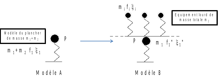
Figure 2: Model Descriptions
We define the following notations:
\({\mathrm{\omega }}_{1}=\sqrt{\frac{{k}_{1}}{{m}_{1}+{m}_{2}}}\)
\({f}_{1}=\frac{1}{2\mathrm{\pi }}\sqrt{\frac{{k}_{1}}{{m}_{1}+{m}_{2}}}\)
\({C}_{1}\) refers to the damping coefficient
\({\xi }_{1}\mathrm{=}\frac{{C}_{1}}{2({m}_{1}+{m}_{2}){\omega }_{1}}\)
\({f}_{1}^{\ast }={f}_{1}\sqrt{1+\mathrm{\lambda }}\)
\({\xi }_{1}^{\mathrm{\ast }}\mathrm{=}{\xi }_{1}\sqrt{1+\lambda }\)
\(\lambda \mathrm{=}\frac{{m}_{2}}{{m}_{1}}\)
\({f}_{i}\mathrm{\in }\mathrm{0,40}\mathit{Hz}\)
\({m}_{i}\mathrm{=}{\alpha }_{i}{m}_{2}\)
\({\Sigma }_{i}{\alpha }_{i}\mathrm{=}1\)
\({\lambda }_{i}\mathrm{=}{\alpha }_{i}\lambda\)
In these notations, we have designated \({\alpha }_{i}\) the effective unit masses associated with each heavy equipment mode and \({\lambda }_{i}\) the mass ratio associated with each of these modes. We will note \(N\) the total number of oscillators constituting the equipment arranged on the floor.
In model A, the oscillator has mass \({m}_{2}+{m}_{1}\) because we consider that the raw accelerogram, calculated during a prior transient analysis, takes into account the added masses. This therefore assumes that the finite element floor model integrates the added masses of heavy equipment.
The calculations required to change the floor spectra are carried out as follows:
Identification of the parameters (frequency \({f}_{1}\) and damping \({\xi }_{1}\) of the support; depreciation \({\xi }_{i}\) of the heavy equipment, mass ratio \(\lambda\), effective unit masses \({\alpha }_{i}\) and frequencies \({\lambda }_{i}\));
Reading the accelerogram at the studied floor point \(\ddot{x}(t)\);
Accelerogram Fourier transform, \(\stackrel{ˆ}{\ddot{x}}(\omega )\);
Calculation of the transfer function between the movement of the mass \({m}_{1}\) in model A and in model B (see Figure 2), \(H(\omega )\);
Product \(\stackrel{ˆ}{\ddot{x}}(\omega )H(\omega )\);
Inverse Fourier transform, \(\ddot{y}(t)\);
Calculation of the spectrum associated with \(\ddot{y}(t)\) with the desired damping \(\xi\).
After calculations, we obtain a series of spectra with the desired damping values. These spectra constitute the corrected floor spectra to be included in the spectra collections. The calculation can be carried out for several points on the floor.
2.2. Calculation of transfer functions#
In this section, we propose to develop the equations leading to the correction of floor spectra by IPM.
The transfer function between the points P in models A and B, see Figure 2 and Figure 3, is equal to the transfer function between the base and the point P in model B divided by the transfer function between the base and the point P in model A.
2.2.1. Transfer function for model B#
Below are the equations of motion for an excitation \({\ddot{x}}_{b}\) at the base of model B:
And:
For a harmonic solicitation of pulsation \(p\) with an amplitude \({\widehat{x}}_{b}\), the equations are written:
And:
: label: eq-4
{m} _ {1} {p} ^ {2} {widehat {2}} {widehat {x}}} _ {1} {widehat {x}}} _ {1}} _ {1} +sum _ {2}} +sum _ {1}} +sum _ {x}} +sum _ {x}} _ {1} - {widehat {x}} _ {i}) + {k}} _ {1} {x} _ {1} +sum _ {i=mathrm {2,} N} {k} {k} _ {k} _ {i} _ {i}) _ {i} _ {1} - {widehat {x}} _ {i}) = {m} _ {1}) = {m} _ {1}) = {m} _ {1}) = {m} _ {1} {p} ^ {2} {widehat {x}} _ {b}
That can be rewritten:
: label: eq-5
(- {p} ^ {2} +2mathit {ip}} {mathrm {omega}}} _ {i} {mathrm {xi}} _ {i} + {mathrm {omega}}} _ {omega}} _ {omega}} _ {i} -2 (2mathit {ip} {omega}} + {mathrm {omega}} _ {ip}} + {mathrm {omega}}} _ {i} -2 (2mathit {ip}} {omega}} + {mathrm {omega}}} _ {i}} + {mathrm {omega}}} + {mathrm {omega}}} _ {i}} + {mathrm {omega}} _ {i} + {mathrm {omega}}} _ {i} ^ {2}) {x} _ {1} = {p} ^ {2} {widehat {x}}} _ {b}
And:
From the equation, we get:
The following notations are defined:
: label: EQ-None
{Delta} _ {i}mathrm {=}mathrm {=}mathrm {-} {p} ^ {2} +mathrm {2ip} {omega} _ {xi} _ {xi} _ {xi} _ {i}} _ {i} ^ {2} _ {i} {overline {x}} _ {j} =frac {{widehat {x}} _ {j}} {{widehat {x}}} _ {b}} _ {b}} overline {{x} _ {i}} =frac {({mathrm {Delta}}} _ {i} + {p} ^ {2})} {{mathrm {Delta}}} _ {i}}} {i}} {i}} {i}} {{i}} _ {i} _ {i} _ {i} _ {1}} +frac {{p} ^ {2}}} {{mathrm {Delta}}} _ {i}}
Using these notations in the equation, we get:
By defining the absolute displacement by \({X}_{i}={\widehat{x}}_{1}+{\widehat{x}}_{b}\), the transfer function at point 2 is equal to:
2.2.2. Transfer function in model A#
With the same notations only for the simple oscillator representing the support in model A:
And:
For a harmonic solicitation of pulsation \(p\) with an amplitude \({\widehat{x}}_{b}\), the equations are written:
By defining the absolute displacement by \({X}_{1}={\widehat{x}}_{1}+{\widehat{x}}_{b}\), the transfer function at point 2 is equal to:
2.2.3. Full transfer function#
The total transfer function \(H(\omega )\) is then calculated by performing the simple ratio between \({T}_{A}\) and \({T}_{B}\):
We check that when \(\lambda \mathrm{=}0\) or \({f}_{i}\to \mathrm{\infty }\), for \(i\mathrm{\in }\mathrm{[}2;N\mathrm{]}\), then \(H(\omega )\mathrm{=}1\); there is therefore, in these two cases, no impact on the raw input spectrum.
2.2.4. Initial conditions#
The transformation of the acceleration of node P between model A and B assumes that the initial conditions are the same between these two models.
It is verified that these conditions are zero by comparing the initial value with respect to the maximum value of the signal:
:math:`frac{left |
{ddot{x}}_{A}(0)right |
}{mathit{max}(left |
{ddot{x}}_{A}(t)right |
)}<mathit{tol}` |
If this condition is not satisfied and the correction option is chosen, the initial value of the signal of model A is modified to 0.