2. Seismic response by modal recombination

2.1. Formulation reminders

The spectral method of seismic analysis is based on the formulation of the transient dynamic response by modal recombination presented in the documents « Methods of RITZ in linear and nonlinear dynamics » [R5.06.01] and « Seismic analysis by direct method or modal recombination » [R4.05.01].

Let’s summarize the principles of the approach detailed in note [R4.05.01] for a structure represented in discretized form by the matrix system:

\(M\ddot{U}+C\dot{U}+KU=F(t)\) eq 2.1-1

Notations in absolute motion

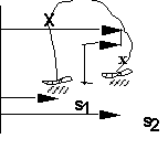
\(U\) represents all the components of the movement (the internal structural degrees of freedom and the degrees of freedom subject to imposed movement): we separate them in the form \(U=(\frac{X}{s})\). The operators describing the structure become: \(K=\left[\begin{array}{cc}{k}_{\mathrm{xx}}& {k}_{\mathrm{xs}}\\ {k}_{\mathrm{sx}}& {k}_{\mathrm{ss}}\end{array}\right]\) \(C=\left[\begin{array}{cc}{c}_{\mathrm{xx}}& {c}_{\mathrm{xs}}\\ {c}_{\mathrm{sx}}& {c}_{\mathrm{ss}}\end{array}\right]\) \(M=\left[\begin{array}{cc}{m}_{\mathrm{xx}}& {m}_{\mathrm{xs}}\\ {m}_{\mathrm{sx}}& {m}_{\mathrm{ss}}\end{array}\right]\)

The problem of relative movement of the structure in relation to the supports with the decomposition Absolute Movement = Relative Movement + Training Movement leads to the introduction of the change of variable \(U=u+E\).

Hypothesis

It is assumed that no excitation force is applied to the structural degrees of freedom, which reduces the second member \(F(t)\) , with the same partition to \(F=(\frac{{0}_{x}}{{r}_{s}})\)

Equation 2.1-1 then becomes:

\(\left[\begin{array}{cc}{m}_{\mathrm{xx}}& {m}_{\mathrm{xs}}\\ {m}_{\mathrm{sx}}& {m}_{\mathrm{ss}}\end{array}\right]\left[\begin{array}{}\ddot{X}\\ \ddot{s}\end{array}\right]+\left[\begin{array}{cc}{c}_{\mathrm{xx}}& {c}_{\mathrm{xs}}\\ {c}_{\mathrm{sx}}& {c}_{\mathrm{ss}}\end{array}\right]\left[\begin{array}{}\dot{X}\\ \dot{s}\end{array}\right]+\left[\begin{array}{cc}{k}_{\mathrm{xx}}& {k}_{\mathrm{xs}}\\ {k}_{\mathrm{sx}}& {k}_{\mathrm{ss}}\end{array}\right]\left[\begin{array}{}X\\ s\end{array}\right]=\left[\begin{array}{}{0}_{x}\\ {r}_{s}\end{array}\right]\) eq. 2.1-2

The first system of equations taken from [éq. 2.1-2]:

\({m}_{\mathrm{xx}}\ddot{X}+{c}_{\mathrm{xx}}\dot{X}+{k}_{\mathrm{xx}}X=-{m}_{\mathrm{xs}}\ddot{s}-{c}_{\mathrm{xs}}\dot{s}-{k}_{\mathrm{xs}}s\) eq. 2.1-3

allows the determination of the response of the internal structural degrees of freedom, while the second:

\({m}_{\mathrm{sx}}\ddot{X}+{c}_{\mathrm{sx}}\dot{X}+{k}_{\mathrm{sx}}X+{m}_{\mathrm{ss}}\ddot{s}+{c}_{\mathrm{ss}}\dot{s}+{k}_{\mathrm{ss}}s=r\)

allows the determination of reaction \(r(t)\) between the structure and its supports.

Notations in relative movement

We decompose the motion vector \(U=(\frac{X}{s})\) into the sum of two vectors \(u\) and \(E\) with:

\(E=(\frac{{e}_{\mathrm{xs}}{s}_{x}}{{s}_{x}})\) the movement of static deformation of the structure under the effect of the movements imposed on the supports, which is called driving movement,

and \(u=(\frac{{x}_{s}}{{0}_{s}})\) the residual deformation movement of the structure with respect to the previous deformation to obtain the absolute deformation \(U=(\frac{X}{s})\).

The vector \({e}_{\mathrm{xs}}{s}_{s}\) is obtained by carrying out the static raising, on the internal degrees of freedom of the structure, of the displacements imposed on the supports either (using the first line of equation 2.1-2 and by eliminating the dynamic components): \({e}_{\mathrm{xs}}{s}_{s}=-{k}_{\mathrm{xx}}^{\text{-1}}{k}_{\mathrm{xs}}{s}_{s}\), or \({e}_{\mathrm{xx}}=-{k}_{\mathrm{xx}}^{\text{-1}}{k}_{\mathrm{xs}}\).

The transition from absolute to relative motion can also be written by introducing the passage operator \(\Psi\):

\(U=(\frac{X}{s})=u+E=(\frac{{x}_{s}}{{0}_{s}})+(\frac{{e}_{\mathrm{xs}}{s}_{s}}{{s}_{s}})=\Psi (\frac{{x}_{s}}{{s}_{s}})\) with \(\Psi =\left[\begin{array}{cc}{I}_{\mathrm{xx}}& {e}_{\mathrm{xs}}\\ {0}_{\mathrm{sx}}& {I}_{\mathrm{ss}}\end{array}\right]\)

The [éq. 2.2.1-1] system then takes the general form:

\(\mathrm{M}\Psi (\frac{\ddot{{\mathrm{x}}_{\mathrm{x}}}}{\ddot{{\mathrm{s}}_{\mathrm{s}}}})+C\Psi (\frac{\dot{{\mathrm{x}}_{\mathrm{x}}}}{\dot{{\mathrm{s}}_{\mathrm{s}}}})+\mathrm{K}\Psi (\frac{{\mathrm{x}}_{\mathrm{x}}}{{\mathrm{s}}_{\mathrm{s}}})\mathrm{=}(\frac{{0}_{\mathrm{x}}}{{\mathrm{r}}_{\mathrm{s}}})\) eq 2.1-4

2.1.1. Multiple imposed movement: multi-support

This situation corresponds to a discrete number of points of connection of the structure to supports subject to different imposed displacements.

Let’s first look at the quasistatic response \({X}^{\mathrm{qs}}\) for structural degrees of freedom. So, \({e}_{\mathrm{xs}}={\varphi }_{s}\), where the matrix \({\varphi }_{s}\) refers to the matrix of static modes reduced to structural degrees of freedom.

So we get: \({X}^{\mathrm{qs}}={\varphi }_{s}s\)

The \({\varphi }_{s}\) matrix includes \(6{n}_{\mathrm{appuis}}\) static modes for structural models and 3 times the number of supports for continuous media models. Each static mode \({\varphi }_{s}=-{k}_{\mathrm{xx}}^{\text{-1}}{k}_{{\mathrm{xs}}_{j}}\) is an attachment mode, corresponding to a displacement imposed unitary on a support component, the other components being zero, and produced by the operator MODE_STATIQUE [28].

The change of frame of reference can then be expressed by:

\(U=(\frac{X}{s})=(\frac{{x}_{s}}{{0}_{s}})+(\frac{{\varphi }_{s}{s}_{s}}{{s}_{s}})\)

The absolute answer is then written in the form: \(U=\left[\begin{array}{cc}{I}_{\mathrm{xx}}& {\varphi }_{s}\\ {0}_{\mathrm{sx}}& {I}_{\mathrm{ss}}\end{array}\right]\left[\begin{array}{}{x}_{x}\\ {s}_{s}\end{array}\right]\)

where \(I\) designates the identity matrix, \({x}_{x}\) the vector of the relative displacements of the structure with respect to the supports, and \(\left[\begin{array}{cc}{I}_{\mathrm{xx}}& {\varphi }_{s}\\ {0}_{\mathrm{sx}}& {I}_{\mathrm{ss}}\end{array}\right]=\Psi\) is the matrix for the transition from absolute to relative movement.

The [éq. 2.1-3] system thus becomes:

\(\left[\begin{array}{cc}{m}_{\mathrm{xx}}& {m}_{\mathrm{xs}}\\ {m}_{\mathrm{sx}}& {m}_{\mathrm{ss}}\end{array}\right]\left[\begin{array}{cc}{I}_{\mathrm{xx}}& {\varphi }_{s}\\ {0}_{\mathrm{sx}}& {I}_{\mathrm{ss}}\end{array}\right]\left[\begin{array}{}\ddot{{x}_{x}}\\ \ddot{{s}_{s}}\end{array}\right]+\left[\begin{array}{cc}{c}_{\mathrm{xx}}& {c}_{\mathrm{xs}}\\ {c}_{\mathrm{sx}}& {c}_{\mathrm{ss}}\end{array}\right]\left[\begin{array}{cc}{I}_{\mathrm{xx}}& {\varphi }_{s}\\ {0}_{\mathrm{sx}}& {I}_{\mathrm{ss}}\end{array}\right]\left[\begin{array}{}\dot{{x}_{x}}\\ \dot{{s}_{s}}\end{array}\right]+\left[\begin{array}{cc}{k}_{\mathrm{xx}}& {k}_{\mathrm{xs}}\\ {k}_{\mathrm{sx}}& {k}_{\mathrm{ss}}\end{array}\right]\left[\begin{array}{cc}{I}_{\mathrm{xx}}& {\varphi }_{s}\\ {0}_{\mathrm{sx}}& {I}_{\mathrm{ss}}\end{array}\right]\left[\begin{array}{}{x}_{x}\\ {s}_{s}\end{array}\right]=\left[\begin{array}{}{0}_{x}\\ {r}_{s}\end{array}\right]\) eq 2.1.1-1

The first equation of this system is written as:

\({m}_{\mathrm{xx}}\ddot{{x}_{x}}+{c}_{\mathrm{xx}}\dot{{x}_{x}}+{k}_{\mathrm{xx}}{x}_{x}=-({m}_{\mathrm{xx}}{\varphi }_{s}+{m}_{\mathrm{xs}})\ddot{{s}_{s}}-({c}_{\mathrm{xx}}{\varphi }_{s}+{c}_{\mathrm{xs}})\dot{{s}_{s}}-({k}_{\mathrm{xx}}{\varphi }_{s}+{k}_{\mathrm{xs}}){s}_{s}\)

The diagonalization of the stiffness term is acquired:

\(\left[\begin{array}{cc}{k}_{\mathrm{xx}}& {k}_{\mathrm{xs}}\\ {k}_{\mathrm{sx}}& {k}_{\mathrm{ss}}\end{array}\right]\left[\begin{array}{}{\varphi }_{s}\\ {I}_{\mathrm{ss}}\end{array}\right]=\left[\begin{array}{}{0}_{x}\\ {r}_{s}\end{array}\right]\)

With regard to damping terms, decoupling is only achieved if damping is proportional to stiffness, a commonly accepted hypothesis.

This makes it possible to decouple the [éq 2.1.1-1] system:

\({m}_{\mathrm{xx}}\ddot{{x}_{x}}+{c}_{\mathrm{xx}}\dot{{x}_{x}}+{k}_{\mathrm{xx}}{x}_{x}={g}_{x}(t)\) eq 2.1.1-2

with \({g}_{x}(t)=-{m}_{\mathrm{xx}}({\varphi }_{s}+{m}_{\mathrm{xx}}^{\text{-1}}{m}_{\mathrm{xs}}){\ddot{s}}_{s}=-{m}_{\mathrm{xx}}{\ddot{x}}^{\mathrm{qs}}-{m}_{\mathrm{xs}}{\ddot{s}}_{s}\)

The equivalent load \({g}_{x}(t)\) is due to the opposite of the sum of the acceleration of the supports and the acceleration relative to the static modes.

This formulation should be interpreted as the decomposition of the movement of the structure into a driving movement corresponding to an instantaneous static deformation (differential displacement of the supports) and a relative movement corresponding to the inertial effects around this new static deformation.

This interpretation is in accordance with the classification of stresses defined by construction rules (ASME, RCC -M):

• the stresses induced by relative motion are, as for static stresses, primary stresses (inertia effects),

• the stresses induced by the differential movements of the supports, which are classified as secondary stresses.

The response of the structural degrees of freedom being thus determined, the second equation of the [éq. 2.1.1.-1] system makes it possible to obtain reaction \(s(t)\).

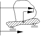
2.1.2. Single imposed movement: mono-support

The training movement then corresponds to a rigid body movement noted \(\left[\begin{array}{}{\varphi }_{R}\\ {s}_{R}\end{array}\right]\). Matrix \({\varphi }_{R}\) refers to the matrix grouping together the rigid body modes of the structure reduced to the degrees of freedom of structure.

The structure is subject to this global movement with an acceleration \(\gamma (t)\), on which we superimpose the relative movement of the degrees of freedom of the structure: the absolute acceleration can therefore be written in the form:

\(\ddot{U}=\left[\begin{array}{}\ddot{X}\\ \ddot{s}\end{array}\right]=\left[\begin{array}{}\ddot{{x}_{x}}\\ {0}_{s}\end{array}\right]+\left[\begin{array}{}{\varphi }_{R}\\ {s}_{R}\end{array}\right]\gamma (t)\)

The rigid part of the displacement verifies the relationship: \(\left[\begin{array}{cc}{k}_{\mathrm{xx}}& {k}_{\mathrm{xs}}\\ {k}_{\mathrm{sx}}& {k}_{\mathrm{ss}}\end{array}\right]\left[\begin{array}{}{\varphi }_{R}\\ {s}_{R}\end{array}\right]=0\)

We deduce that: \({\varphi }_{R}={\varphi }_{S}{s}_{R}\)

\(U=(\frac{X}{s})=(\frac{{x}_{s}}{{0}_{s}})+(\frac{{\varphi }_{R}{s}_{x}}{{s}_{s}})\) and \(\Psi =\left[\begin{array}{cc}{I}_{\mathrm{xx}}& {\varphi }_{R}\\ {0}_{\mathrm{sx}}& {I}_{\mathrm{ss}}\end{array}\right]\)

The second member of equation [éq. 2.1.1-2] can then be written in the form:

\({g}_{x}(t)=-{m}_{\mathrm{xx}}({\varphi }_{s}+{m}_{\mathrm{xx}}^{\text{-1}}{m}_{\mathrm{xs}}){\ddot{s}}_{\mathrm{xx}}=-({m}_{\mathrm{xx}}{\varphi }_{R}+{m}_{\mathrm{xs}}{s}_{R})\gamma (t)\) eq. 2.1.2-1

This writing clearly shows that seismic loading only depends on the overall acceleration and inertia associated with rigid body modes.

2.1.3. Summary

The equations [éq 2.1.1-2] and [éq 2.1.2-1] lead to the general form (written without a clue for greater clarity):

\(m\ddot{z}+c\dot{z}+kz=-m({\varphi }_{X}+{m}^{\text{-1}}{m}_{\mathrm{xs}})\ddot{s}=-mO\ddot{s}\) eq 2.1.3-1

The terms \({m}_{\mathrm{xs}}\) correspond to the coupling terms of the mass matrix with the support degrees of freedom: this fraction of the total mass is very low and it is justified to neglect it. Recall that this term is effectively zero for structural models whose mass matrix is diagonal: mass-spring models, models with « lumped mass » elements.

In this case, the simplified formulas are obtained:

• mono-support: \(\mathrm{O}\mathrm{=}{\varphi }_{\mathrm{R}}\) where \({\varphi }_{R}\) are the six solid body modes,

• multi-support: \(O={\varphi }_{s}\) where \({\varphi }_{s}\) are the \(6n\) supports, attachment modes.

The second member \(\mathrm{-}\mathrm{m}\mathrm{O}\) is constructed by the CALC_CHAR_SEISME [U4.63.01] operator.

2.2. Response on a modal basis

2.2.1. Temporal response of a modal oscillator

If the structure studied is represented by its spectrum of real low-frequency eigenmodes \(\varphi\) in an embedded base, solution of \((K-M{\omega }^{2})\varphi =0\) or \((k\mathrm{-}m{\omega }^{2})\varphi \mathrm{=}0\), we can introduce a new transform \(x=\varphi q\) and the system of equations [éq 2.1.3-1] can be written, using the matrix of modal participation factors \(P\):

\(\ddot{\mathrm{q}}+\frac{{\phi }^{\mathrm{T}}\mathrm{c}\phi }{{\phi }^{\mathrm{T}}\mathrm{m}\phi }\dot{\mathrm{q}}+{\omega }^{2}\mathrm{q}=-\frac{{\phi }^{\mathrm{T}}\mathrm{m}\mathrm{O}}{{\phi }^{\mathrm{T}}\mathrm{m}\phi }\ddot{\mathrm{s}}=-\mathrm{P}\ddot{\mathrm{s}}\) eq 2.2.1-1

Hypothesis:

For industrial studies involving seismic analysis by spectral method, we limit ourselves to the case of proportional damping, known as RAYLEIGH, for which we can diagonalize the term \(\frac{{\varphi }^{T}c\varphi }{{\varphi }^{T}m\varphi }=2\xi \omega\). Damping is then represented by a modal dampening \({\xi }_{i}\) that may be different for each mode proper [R4.05.01].

Each specific mode, characterized by the parameters \(({\omega }_{i},{\xi }_{i})\), is assimilated to a simple oscillator whose behavior is represented in the general case by:

\(\ddot{{q}_{i}}+2{\xi }_{i}{\omega }_{i}\dot{{q}_{i}}+{\omega }^{2}{q}_{i}=-{(P\ddot{s})}_{i}\) eq 2.2.1-2

Remember that the \(\ddot{\mathrm{s}}\) are training accelerations.

2.2.2. Modal participation factor in mono-support

When the training movement is unique, [éq 2.2.1-2] becomes:

\(\ddot{{q}_{i}}+2{\xi }_{i}{\omega }_{i}\dot{{q}_{i}}+{\omega }^{2}{q}_{i}=-{p}_{i}\ddot{s}\) eq 2.2.2-1

with

\({p}_{i}=\frac{{\varphi }_{i}^{T}\mathrm{.}\text{m . O}}{{\varphi }_{i}^{\mathrm{T.}}m\mathrm{.}{\varphi }_{i}}=\frac{{\varphi }^{T}\mathrm{.}m\mathrm{.}{\varphi }_{R}}{{\mu }_{i}}\) eq 2.2.2-2

where \({\mu }_{i}\) is the generalized modal mass, which depends on the normalization of the eigenmode. Let us state some properties of modal participation factors \({p}_{i}\) in the case of rigid modes of translation, but extensible to modes of rotation.

• A \({\varphi }_{\mathrm{RX}}\) mode, which we will note \({\delta }_{X}\), to recall that the components in the \(X\) direction are unitary, belongs to the space of dimension \(N\) degrees of freedom whose \(N\) eigenmodes constitute a basis in which \({\delta }_{X}=\sum _{i}{\alpha }_{i}\varphi\).

From the orthogonality properties of the eigenmodes \({\varphi }_{i}^{T}\mathrm{.}m\mathrm{.}{\varphi }_{j}={\mu }_{i}{\delta }_{\mathrm{ij}}\), we identify the coefficients \({\alpha }_{i}\) with the modal participation factors \({p}_{\mathrm{iX}}\) in the direction \(X\) and

\({\delta }_{X}=\sum _{i=\mathrm{1,}\mathrm{...},N}{p}_{\mathrm{iX}}{\varphi }_{i}\) eq 2.2.2-3

• In addition \({\delta }_{X}^{T}\mathrm{.}m\mathrm{.}{\delta }_{X}={m}_{T}\) total mass of the structure trained in the \({\delta }_{X}\) movement, which leads to, having noted \(N\) the total number of degrees of freedom of the system, equal to the number of modes:

\({\delta }_{X}^{T}\mathrm{.}m\mathrm{.}{\delta }_{X}=\sum _{\mathrm{ij}}{p}_{\mathrm{iX}}{p}_{\mathrm{jX}}{\varphi }_{j}^{T}\mathrm{.}m\mathrm{.}{\varphi }_{i}=\sum _{i=\mathrm{1,}\mathrm{...},N}{p}_{\mathrm{iX}}^{2}{\mu }_{i}\) and \({m}_{T}=\sum _{i=\mathrm{1,}\mathrm{...},N}{p}_{\mathrm{iX}}^{2}{\mu }_{i}\) or \(\frac{\sum _{i=\mathrm{1,}\mathrm{...},N}{p}_{\mathrm{iX}}^{2}{\mu }_{i}}{{m}_{T}}=1\) eq 2.2.2-4

The modal parameter \({p}_{\mathrm{iX}}\) depends on the proper mode standard and is accessible, for each mode proper, in the result concept of the mode_meca type under the name FACT_PARTICI_DX; similarly \({p}_{\mathrm{iX}}^{2}{\mu }_{i}\), independent of the standard, is accessible under the name of MASS_EFFE_UN_DX.

2.2.3. Modal participation factor in multi-support

For a multiple imposed movement, [éq 2.2.1-2] becomes:

\(\ddot{{q}_{i}}+2{\xi }_{i}{\omega }_{i}\dot{{q}_{i}}+{\omega }^{2}{q}_{i}=-\sum _{j}{p}_{\mathrm{ij}}\ddot{{s}_{j}}\) eq 2.2.3-1

with

\({p}_{\mathit{ij}}=\frac{{\mathrm{\phi }}_{i}^{T}\mathrm{.}\mathrm{m}\mathrm{.}\mathrm{O}}{{\mathrm{\phi }}_{i}^{T}\mathrm{.}\mathrm{m}\mathrm{.}{\mathrm{\phi }}_{i}}=\frac{{\mathrm{\phi }}_{i}^{T}\mathrm{.}\mathrm{m}\mathrm{.}{\mathrm{\phi }}_{{s}_{j}}}{{\mu }_{i}}\) eq 2.2.3-2

where \({\mu }_{i}\) is the generalized modal mass, which depends on the normalization of the mode proper and \({p}_{\mathrm{ij}}\) can be considered as participation factors relating to the mode \(i\) and to a direction \(j\) of movement imposed by a support.

As before, we can establish [bib4] the two properties:

\({\varphi }_{\mathrm{sj}}=\sum _{i}{p}_{\mathrm{ij}}{\varphi }_{i}\) and \({\varphi }_{\mathrm{sj}}^{T}\mathrm{.}m\mathrm{.}{\varphi }_{\mathrm{sj}}=\sum _{i=\mathrm{1,}\mathrm{...},N}{p}_{\mathrm{ij}}^{2}{\mu }_{i}\) eq 2.2.3-3

At this stage, we are not making any assumption of dependence between the different terms \({p}_{\mathrm{ij}}\). Recall that components \(\ddot{{s}_{j}}\) express the drive acceleration applied to a support direction \(j\).

Participation factors \({p}_{\mathrm{ij}}\) are not built independently and only appear as intermediate variables in the COMB_SISM_MODAL [U4.84.01] command.

The participation factor can also be estimated using the following formula:

\({p}_{\mathit{ij}}=\frac{{\mathrm{\phi }}_{i}^{T}\mathrm{.}\mathrm{m}\mathrm{.}\mathrm{O}}{{\mathrm{\phi }}_{i}^{T}\mathrm{.}\mathrm{m}\mathrm{.}{\mathrm{\phi }}_{i}}=\frac{-{\mathit{Reac}}_{\mathit{ij}}}{{\mu }_{i}{\omega }_{i}^{2}}\)

where \({\mathit{Reac}}_{\mathit{ij}}\) is the value of the reaction in support \(j\) in the \(i\) mode.