1. Oscillator spectrum concept

The spectral method for studying the response of a structure under the effect of imposed seismic-type movements is based on the concept of the oscillator spectrum of an earthquake accelerogram.

1.1. Imposed movement defined by an accelerogram A (t)

For an imposed movement \(s\) of the seismic type, we can treat the problem in absolute displacement \(X\) or in relative displacement \(x\) such as: \(X=x+s\). The general equations of motion of a simple oscillator are then written as:

	Absolute movement \(m\ddot{X}+c\dot{X}+kX=c\dot{s}+ks\)	Relative movement \(m\ddot{x}+c\dot{x}+kx=-m\ddot{s}\)

We use the formulation based on the relative movement for two main reasons:

• the seismic analysis of structures uses the stresses induced by the inertial effects of the earthquake, stresses calculated from the deformations of the structure which are expressed from the relative displacements;

• the characterization of the excitation signal can in this case be reduced to the accelerogram of earthquake \(\ddot{s}=A(t)\), a quantity provided directly by the seismographs. Movement \(s\) and speed \(\dot{s}\) signals are generally not available in geotechnical databases.

For the determination of the response of a simple oscillator to an imposed movement and the conventional notations, refer to Appendix 2 [R4.05.03 Annexe 2].

If the earthquake is defined by an accelerogram \(A(t)\), with absolute acceleration applied to the base, the reduced equation is in this case:

\(\ddot{x}+2\xi {\omega }_{0}\dot{x}+{\omega }_{o}^{2}x=-\ddot{s}=-A(t)\) eq 1.1-1

The solution to this problem is the integral of DUHAMEL shown in Appendix A [éqA3.3-1]:

\(x(t)=\frac{1}{\omega {\text{'}}_{0}}{\int }_{0}^{t}A(\tau ){e}^{-\xi {\omega }_{0}(t-\tau )}\mathrm{sin}\omega {\text{'}}_{0}(t-\tau )d\tau =f(A,\xi ,\omega {\text{'}}_{0})\) eq 1.1-2

\(\omega {\text{'}}_{0}={\omega }_{0}\sqrt{1-{\xi }^{2}}\)

1.2. Accelerogram oscillator spectrum

The concept of oscillator spectrum was introduced initially to compare the effects of different accelerograms with each other. The FOURIER spectrum of a \(A(t)\) signal provides information on its frequency content. The response of a mechanical system to a movement imposed at the base depends largely on the dynamic characteristics of this system: natural frequencies and reduced damping \((\xi ,{\omega \text{'}}_{0})\). Appendix A details this aspect.

If we want to know the maximum value of the response of a simple oscillator to the parameters, \((A,\xi ,{\omega \text{'}}_{0})\) we must evaluate the integral of DUHAMEL which provides the response of the oscillator [éq 1.1-2] to an excitation imposed at the base.

Figure 1.2-a: Accelerograph

1.2.1. Relative displacement oscillator spectrum

From the integral of DUHAMEL, we can define the oscillator spectrum of an accelerogram \(A(t)\) as the function of the maximum values of the relative displacement \(x(t)=f(A,\xi ,{\omega \text{'}}_{0})\) for each value of \((\xi ,{\omega \text{'}}_{0})\) by recalling that: \(\omega {\text{'}}_{0}={\omega }_{0}\sqrt{(1-{\xi }^{2})}\).

\(\mathrm{Srox}(A,\xi ,\omega {\text{'}}_{0})={\mid x(t)\mid }_{\mathrm{max}}\)

\(x(t)=\frac{1}{\omega {\text{'}}_{0}}{\int }_{0}^{t}A(\tau ){e}^{-\xi {\omega }_{0}(t-\tau )}\mathrm{sin}\omega {\text{'}}_{0}(t-\tau )d\tau =f(A,\xi ,\omega {\text{'}}_{0})\)

It can be seen, in figure [Figure 1.2.1-a], that beyond a certain frequency (\(35\mathit{Hz}\) here), called spectrum cutoff frequency, there is no significant dynamic amplification: the relative displacement is zero.

Figure 1.2.1-a: Oscillator spectrum in relative displacement

1.2.2. Relative pseudo-speed oscillator spectrum

For structures with low reduced damping \(\xi <0.2=20\text{\%}\), for which it is acceptable to assimilate \({\omega }_{0}\) and \(\omega {\text{'}}_{0}\), the pseudo-speed spectrum defined by:

\(\mathrm{Sro}\dot{x}(A,\xi ,{\omega }_{0})={\omega }_{0}\mathrm{Srox}(A,\xi ,{\omega }_{0})={\omega }_{0}{\mid x(t)\mid }_{\mathrm{max}}\)

The pseudospeed is the value of the speed which gives a value of the kinetic energy of the mass of the oscillator equal to that of the maximum deformation energy of the spring:

\({E}_{c}=\frac{1}{2}m{(\dot{x}(t))}^{2}=\frac{1}{2}m{\left[\mathrm{Sro}\dot{x}(A,\xi ,{\omega }_{0})\right]}^{2}=\frac{1}{2}m{\omega }_{0}^{2}{\mid x(t)\mid }_{\mathrm{max}}^{2}=\frac{1}{2}k{\mid x(t)\mid }_{\mathrm{max}}^{2}={E}_{p}\)

Figure 1.2.2-a: Oscillator spectrum in pseudo-relative velocity

1.2.3. Absolute pseudo-acceleration oscillator spectrum

Likewise, for low reduced damping, it is possible to define the pseudo-acceleration spectrum defined by:

\(\mathrm{Sro}\ddot{x}(A,\xi ,{\omega }_{0})={\omega }_{O}^{2}\mathrm{Srox}(A,\xi ,{\omega }_{0})={\omega }_{0}^{2}{\mid x(t)\mid }_{\mathrm{max}}\)

Figure 1.2.3-a: Oscillator spectrum in pseudo-absolute acceleration

The advantage of this pseudo-acceleration spectrum lies in the fact that \(\mathrm{Sro}\stackrel{\cdots }{x}(A,\xi ,{\omega }_{0})\) is a good approximation of the absolute acceleration maximum \(\ddot{X}(t)\). In fact, at the moment when the relative displacement is maximum, the relative speed is canceled and the reduced equation is written \(\ddot{x}+0+{\omega }_{0}^{2}{x}_{\mathrm{max}}=-\ddot{s}\), which shows us that

\({\mid \ddot{X}\mid }_{\mathrm{max}}={\mid \ddot{x}+\ddot{s}\mid }_{\mathrm{max}}=\mid {\omega }_{0}^{2}{x}_{\mathrm{max}}\mid ={\omega }_{O}^{2}\mathrm{Srox}(A,\xi ,{\omega }_{0})=\mathrm{Sro}\ddot{x}(A,\xi ,{\omega }_{0})\)

For this reason, this oscillator spectrum is called absolute pseudo-acceleration spectrum.

The asymptote of this high-frequency spectrum (zero-period acceleration) corresponds to the response of a natural, i.e. very rigid, high-frequency oscillator. In this case, the mass tends to fully follow the movement imposed from the base. This asymptote therefore corresponds to the maximum acceleration \({\mid A(t)\mid }_{\mathrm{max}}\) of the imposed movement (ground or oscillator attachment point). In practice, it is reached from the cutoff frequency of the spectrum. For this reason, we say that an accelerogram is set to, for example, \(0.15g\), when its maximum amplitude and its zero period absolute pseudo-acceleration oscillator spectrum are equal to \(0.15g\).

1.3. Determining the oscillator spectrum

The determination of the oscillator spectrum of an accelerogram \(A(t)\) is available in the operator CALC_FONCTION [U6.34.04] with the keyword SPEC_OSCI: it is obtained by numerical integration of the equation of DUHAMEL by the method of NIGAM [R5.05.01]. This command provides the absolute pseudo-acceleration spectrum and, upon request, the pseudo-speed spectrum or the relative displacement spectrum.

1.4. Representation and use of oscillator spectra

1.4.1. Tri-logarithmic representation

Oscillator response spectra are commonly represented by tri-logarithmic graphs that allow the three quantities to be read on a single graph: relative displacement, relative pseudo-speed, and absolute pseudo-acceleration.

This representation is obtained by drawing the relative pseudo-speed spectrum \(\mathrm{Sro}\dot{x}\) in coordinates \(\mathrm{log}-\mathrm{log}\) such as \(\text{log}\mathrm{Sro}\dot{x}=f(\text{log}{\omega }_{0})\), on which two complementary graduations are transferred to \(\pm 45°\) if the logarithmic scale is the same on both axes:

• a logarithmic scale to \(+45°\) to measure the relative movements \(\text{log}\mathrm{Sro}x=\text{log}(\frac{\mathrm{Sro}\dot{x}}{{\omega }_{0}})=\text{log}\mathrm{Sro}\dot{x}-\mathrm{log}{\omega }_{0}\)

• a logarithmic scale to \(–45°\) to measure absolute accelerations \(\text{log}\mathrm{Sro}\ddot{x}=\text{log}({\omega }_{0}\mathrm{Sro}\dot{x})=\text{log}\mathrm{Sro}\dot{x}+\mathrm{log}{\omega }_{0}\)

\(\begin{array}{}f=3\mathrm{Hz}\\ \dot{x}=1m/s\\ x=\frac{\dot{x}}{\omega }=\frac{1}{6\pi }=0.05305\\ \dot{x}=\omega x=6\pi =18.849\end{array}\)

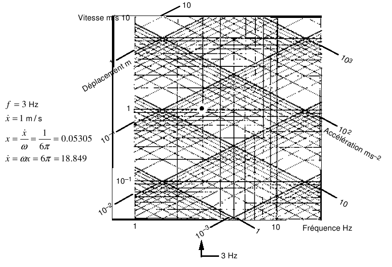
Figure 1.4.1-a: Tri-logarithmic representation

1.4.2. Using oscillator spectra

To evaluate the maximum response of a modal oscillator \(({\omega }_{i},{\xi }_{i})\) to an accelerogram \(A(t)\), the absolute pseudo-acceleration spectrum are used.

It is represented in Code_Aster by a tablecloth consisting of several functions \(\mathrm{Sro}\ddot{x}=f(\mathrm{freq})\) to \({\xi }_{n}=\mathrm{cte}\).

We use linear interpolation on the reduced damping for \({\xi }_{n}<{\xi }_{i}<{\xi }_{n+1}\) because the dynamic amplification at resonance for \(\omega ={\omega }_{0}\) (i.e. \(\eta =1\)) is equal to \(\frac{{x}_{m}}{{s}_{0}}=\frac{1}{2{\xi }_{i}}\) [éq A2.2-3].

The variation in the modulus of the response in the vicinity of resonance also justifies logarithmic interpolation for \({\omega }_{m}<{\omega }_{i}<{\omega }_{m+1}\). The oscillator spectrum must be represented with a frequency discretization that is sufficiently fine to limit the effects of interpolation.

1.5. Oscillator spectra used for studies

For studies of industrial installations, such as nuclear power plants, seismic analysis leads to the establishment of several models:

• a building structure design model to determine:

• accidental stresses for the design of the frames of these buildings;

• the movements imposed at the attachment points of the equipment (reactor vessel, supports of pipe networks, electrical cabinets, etc.) at different levels of buildings;

• study models to verify each piece of equipment subjected to imposed movements amplified by the dynamic behavior of buildings.

1.5.1. Design soil spectrum and building verification

At this stage, the equipment is only known as inertial overloads and it can be assumed that it does not provide any rigidity to the building. In this case, the structures are subject to a soil spectrum.

The frequency content of an oscillator spectrum reflects that of the accelerogram used and is therefore « marked » by the properties of the ground at the place of recording. To develop the ground spectrum at the project stage, it is therefore recommended to establish the oscillator spectra for several accelerograms and to build an envelope spectrum that smoothes the anti-resonances.

Figure 1.5.1-a: Soil spectrum for a project

Note:

In many cases, we do not know the rotational movement imposed by the earthquake, since the known earthquake accelerograms come from seismograph recordings, sensors with a degree of freedom of translation.

1.5.2. Equipment verification floor spectrum

The study of the dynamic behavior of equipment subjected to the movements imposed by the support structure at the points of support is possible from the accelerograms of response at these points, results of the transitory analysis of the behavior of the building: these accelerograms, called floor accelerometers, make it possible to construct floor spectra.

To verify the equipment, it is possible to limit ourselves to a spectral analysis based on floor spectra and the differential movements imposed on the supports.

The floor spectra are representative of the dynamic amplification provided by the support structure: smoothing the spectrum can be useful to take into account the uncertainty about the position of the natural frequencies of the building, but care will be taken to maintain realistic margins, since the ground spectrum is already an increase in seismic stress. The oscillator spectrum must be represented with a frequency discretization that is fine enough to « pick up » the resonances of the structure.

Note:

Techniques for the direct determination of floor spectra, based on the soil spectrum and structural modes, have been developed [bib1], but are not currently available in Code_Aster.