4. Integration#
The laws of friction envisaged are perfect adhesion, sliding without friction and Coulomb friction with a threshold allowing to find the tension profiles given by BPEL (or by ETCC since the 2 codes use equivalent formulas). These three scenarios can be used with the law of behavior CABLE_GAINE_FROT.
The addition of new friction laws adapted to other regulations is possible.
At a given Gauss point, the integration of laws consists in determining \({\delta }_{g}\). To do this, we look for the intersection point between the line representative of equation \({t}_{g}\mathrm{=}{\lambda }_{g}+r({g}_{g}\mathrm{-}{\delta }_{g})\) (green curve in the figures,,) and the curve representative of the derivative of \(\Pi ({\delta }_{g})\) (blue curve in the figures).
Note: in the following paragraphs, we adopt a notation on movements in order not to burden the ratings rather than on the increments of movements as is really the case.
4.1. Perfect grip#
In the first case, corresponding to perfect adherence, we have:
\(\Pi ({\delta }_{g})\mathrm{=}{I}_{R⁺}({\delta }_{g})+{I}_{R⁻}({\delta }_{g})\)
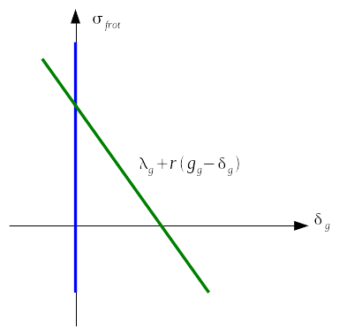
Figure 4-1: Graphical interpretation of the integration of the law of perfect adherence
The solution is: \({\delta }_{g}=0\)
4.2. Frictionless sliding#
In the second case, sliding without friction, we have:
\(\Pi ({\delta }_{g})\mathrm{=}0\)
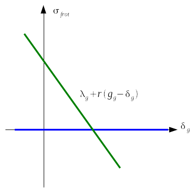
Figure 4-2: Graphical interpretation of the integration of the perfect sliding law
The solution verifies:
\(0\mathrm{=}{\lambda }_{g}+r({g}_{g}\mathrm{-}{\delta }_{g})\)
whence
\({\delta }_{g}\mathrm{=}{g}_{g}+\frac{{\lambda }_{g}}{r}\)
4.2.1. Sliding with friction (BPEL)#
This law makes it possible to take into account rectilinear friction and curved friction. The tensions imposed by BPEL are found by choosing the threshold of Coulomb’s law \({\sigma }_{c}\) as follows:
\({\sigma }_{c}\mathrm{=}\mathrm{-}(\varphi +f\frac{\mathrm{\partial }\alpha }{\mathrm{\partial }s})N\)
with the notations of [R7.01.02] §2.2.2 that we recall:
\(f\) the coefficient of friction of the cable on the partly curved concrete, in \({\mathit{rad}}^{\mathrm{-}1}\),
\(\varphi\) the coefficient of friction per unit length, in \({m}^{\mathrm{-}1}\),
\(\alpha\) the cumulative angular deviation.
and with \(N\) the normal effort.
In fact, considering that the cable slides over its entire length during tension and noting \(s\) on the curvilinear abscissa along the cable, the balance of the cable is written:
\(\frac{\mathit{dN}}{\mathit{ds}}\mathrm{=}\mathrm{-}(\varphi +f\frac{\mathrm{\partial }\alpha }{\mathrm{\partial }s})N\)
Hence by integration:
\(N\mathrm{=}{N}_{0}\mathrm{exp}(\mathrm{-}(\varphi s+f\alpha (s)))\)
We then recognize the expression of cable tension in the presence of rectilinear friction of BPEL ([R7.01.02] §2.2.2).
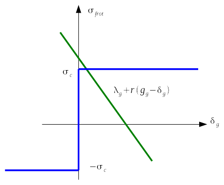
Figure 4-3: Graphical interpretation of the integration of the law of friction BPEL
To write the solution, there are 3 scenarios:
if \(∣({\lambda }_{g}+{\mathit{rg}}_{g})∣\mathrm{\le }{\sigma }_{c}\): \({\delta }_{g}=0\)
if \({\lambda }_{g}+{\mathit{rg}}_{g}>{\sigma }_{c}\): \({\delta }_{g}\mathrm{=}{g}_{g}+\frac{{\lambda }_{g}\mathrm{-}{\sigma }_{c}}{r}\)
if \({\lambda }_{g}+{\mathit{rg}}_{g}<\mathrm{-}{\sigma }_{c}\): \({\delta }_{g}\mathrm{=}{g}_{g}+\frac{{\lambda }_{g}+{\sigma }_{c}}{r}\)
The case where normal force \(N\) is negative should not normally occur for prestress cable problems. However, it can happen to have very slightly negative values. We make the choice to adopt slippery behavior in such a case.
Note 1: by introducing such a dependence of slip on tension in the cable, the contribution of the variation of this tension to slippage \(\frac{\partial {\delta }_{g}}{\partial N}\) induces a non-symmetric matrix.
Note 2: In order for curved friction to be taken into account at the elementary level, it is imperative that the curvature of the cable be transcribed into its constituent elements, i.e. the three knots of mesh SEG3 must not be aligned.