2. Discretization of the finite element#
Preliminary remark:
The finite element envisaged models the interface of the cable with its sheath and the cable itself. It would have been possible to model the cable-sheath interface separately (with a finite interface element) and the cable itself (with a finite cable element), however, as will be seen below, the law of friction behavior requires knowledge of the tension in the cable, so it is advantageous to have the interface and the cable in the same element. In addition, as will be seen below, the proposed modeling is based on quadratic elements, so it is not possible to reuse the existing BARRE element.
The finite element envisaged is linear (geometric support in the form of segments), in contrast to the interface elements which are surface or solid.
It is considered to represent a cable immersed in a volume (of concrete) \(\mathrm{3D}\). As a result, the degrees of freedom are:
sheath movements (3 degrees of freedom): \({u}_{\mathit{gaine}}\)
the relative longitudinal displacement of the cable in sheath \(g\)
and the Lagrange multiplier \(\lambda\).
In a manner similar to interface elements, relative slippage \(\delta\) is discretized at Gauss points and then eliminated by static condensation. The interpolation adopted is P2 for the movements (of the duct and the cable) and P1 for the Lagrange multiplier. The supporting geometric elements will therefore be SEG3. Constraint \(g=\delta\) is imposed in a weak sense.
The Gauss points chosen are the same as for the under-integrated interface element, i.e. 2 integration points (unlike the interface elements presented in [R3.06.13], the fact that the cable only has longitudinal displacements controlled by the stiffness of the cable does not require the use of 3-point Gauss integration. This point was verified during the tests). The following figure shows all of this information.
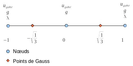
Figure 2-1: discretization of element CABLE_GAINE