5. Skeleton assembly element#
The skeleton assembly element is a generalization of the multi-fiber beam element presented in the previous section. This element consists of an element with beam kinetics, but where lots of fibers are grouped into sub-beams that represent the guide tubes. These sub-beams are themselves multi-fibers, as shown in the figure. This element is only accessible in the context of Euler beam kinematics.
The hypotheses adopted are as follows:
the Euler hypothesis: transverse shear is neglected (this hypothesis is verified for strong movements);
the element carries the usual degrees of freedom of movement and rotation of the beams as well as three additional degrees of freedom modeling the rotation of the grid linking the guide tubes kinematically;
the rotations in all the beams are all the same;
the skeleton element takes into account the effects of thermal expansion, gravity and, in a simplified manner, twisting.
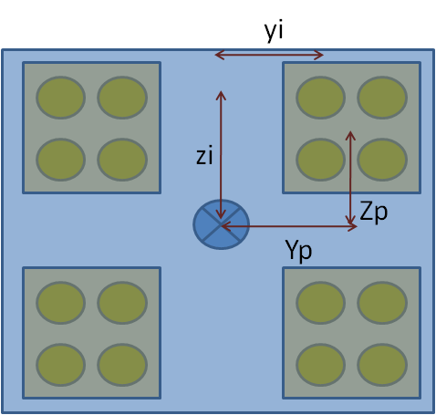
Figure 5-a : Example of a multi-beam section consisting of 4 sub-beams described by a rectangular section. In the example, the sub-beams are made up of 4 fibers.
5.1. Finite element kinematics#
We consider here a structural element describing the skeleton of a fuel assembly consisting of \({N}_{p}\) tube-guides here considered as three-dimensional beams. These guide tubes are linked kinematically to one another by the grids of the fuel assembly, here considered to be a rigid body. Based on these two hypotheses, it is possible to describe all the kinematics of this assembly of beams using nine degrees of freedom, as shown in the Figure:
three degrees of freedom representing the movement of the grid: \(({u}_{x},{u}_{y},{u}_{z})\)
three degrees of freedom describing the rotations of the guide tubes: \(({\mathrm{\theta }}_{x},{\mathrm{\theta }}_{y},{\mathrm{\theta }}_{z})\)
three degrees of freedom modeling the rotation of the grid connecting the guide tubes: \(({\mathrm{\omega }}_{x},{\mathrm{\omega }}_{y},{\mathrm{\omega }}_{z})\)
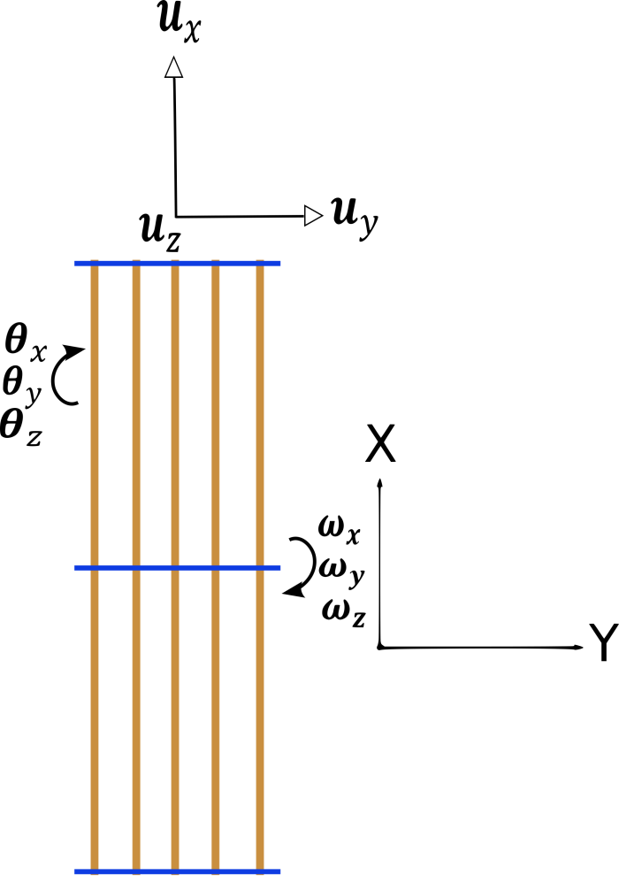
Figure 5.1-a : **Diagram of the fuel assembly element
The position of a guide tube \(i\) in relation to the center of the skeleton of the assembly is described using a pair of real \(({Y}^{i},{Z}^{i})\). Using the usual degrees of freedom (three displacements and three rotations) of an Euler beam in three dimensions and assuming that the rotations in all the beams are the same, the kinematics of guide tube \(i\) is written as:
In addition, in order to use beams with non-linear behavior, the section of the beams is itself described using fibers (numbered from \(1\) to \({N}_{f}\)) and the theory of multifibre beams is used here. Thus, for each beam \(i\) (varying from \(1\) to \({N}_{p}\)), the axial displacement of its fiber \(j\) is a function of the average displacement of the section of the beam, to which is added the displacement imposed by the rotation of the section. Since the theory of beams requires that the cross section of the beams remain straight, the axial displacement field of fiber \(j\) of a guide tube \(i\) is written as:
By injecting the first equation () into it:
Where the quantity \(({y}^{i,j},{z}^{i,j})\) corresponds to the position of the \(j\) fiber of a \(i\) beam in relation to the center of the beam assembly. The axial deformation field of the fiber is subsequently determined by:
: label: eq-4
{mathrm {epsilon}} _ {mathit {xx}}} ^ {i, j}} =frac {partial {u} _ {x} ^ {i, j}} {partial x}}} {partial x}} = {u} _ {x}} = {u} _ {x}} ^ {i} = {u} _ {x}} = {u} _ {x}} = {u} _ {x}} = {u} _ {x}} = {u} _ {x}} = {u} _ {x}} = {u} _ {x}} = {u} _ {x}} = {u} _ {x}}mathrm {.} {mathrm {omega}} _ {z}} ^ {text {“}}left (xright) + {Z} ^ {i}mathrm {.} {mathrm {omega}} _ {y} ^ {text {“}}left (xright) -left ({y} ^ {i, j} - {Y} ^ {i} ^ {i}right)mathrm {.} {mathrm {theta}} _ {z}} ^ {text {“}}left (xright) +left ({z} ^ {i, j} - {Z} ^ {i}right)mathrm {.} - {Z} ^ {i}right)mathrm {.} {mathrm {theta}} _ {y}} ^ {text {“}}left (xright)
The principle is to rely on existing multi-fiber beams by passing the degrees of freedom of the assembly skeleton element to the \(i\) fields of « generalized multi-fiber beam movements » constituting it, using (). By proceeding in this way (i.e. by treating all the beams individually), a « generalized local displacement field » \({U}_{i}\) is determined for each of the beams \(i\). For each of the beams, we thus return to determining the fields using the six « classical » degrees of freedom along the element.
Thus, the generalized deformations \({D}_{i}\) on each of the beams \(i\) are determined with \({D}_{i}=B\mathrm{.}{U}_{i}\) (cf. [R3.08.08]). Once that is done, you can:
determine the uniaxial deformations on the fibers in the same way as for Euler multi-fiber beams;
obtain the constraints by the law of behavior;
determine the generalized forces on the \(i\) beam as for an Euler multi-fiber beam based on the constraints;
assemble the elementary matrix of the assembly skeleton from the matrices of each sub-beam;
finally, it is necessary to build the generalized forces of the assembly element from the generalized forces on the beams \(i\). It will be a question of separating the moments caused by the rotation of the beams and those caused by the rotation of the grid.
The implementation of this finite element is intended as an encapsulation of the multi-fiber Euler beam model.
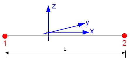
The discretization of the skeleton element is performed on a linear element with two nodes and nine degrees of freedom per node. These degrees of freedom are the three translations \((u,v,w)\) and the six rotations relating to the \(({\mathrm{\theta }}_{x},{\mathrm{\theta }}_{y},{\mathrm{\theta }}_{z})\) beams and the \(({\mathrm{\omega }}_{x},{\mathrm{\omega }}_{y},{\mathrm{\omega }}_{z})\) grids.
\(\left\{\begin{array}{c}{u}_{1}\\ {v}_{1}\\ {w}_{1}\end{array}\begin{array}{c}{\theta }_{{x}_{1}}\\ {\theta }_{{y}_{1}}\\ {\theta }_{{z}_{1}}\end{array}\begin{array}{c}{\mathrm{\omega }}_{{x}_{1}}\\ {\mathrm{\omega }}_{{y}_{1}}\\ {\mathrm{\omega }}_{{z}_{1}}\end{array}\right\}\)
\(\left\{\begin{array}{c}{u}_{2}\\ {v}_{2}\\ {w}_{2}\end{array}\begin{array}{c}{\theta }_{{x}_{2}}\\ {\theta }_{{y}_{2}}\\ {\theta }_{{z}_{2}}\end{array}\begin{array}{c}{\mathrm{\omega }}_{{x}_{2}}\\ {\mathrm{\omega }}_{{y}_{2}}\\ {\mathrm{\omega }}_{{z}_{2}}\end{array}\right\}\)
Figure e5.1-b: Element skeleton .
Since the deformations are local, a local base is constructed at each vertex of the mesh, depending on the element on which we are working. The continuity of the fields of travel is ensured by a change of base, bringing the data back into the global database. In the case of straight beams, the mean line is traditionally placed on the axis \(x\) of the local base, the transverse movements thus taking place in the plane \((y,z)\).
Finally, when we order quantities related to the degrees of freedom of an element in an elementary vector or matrix (therefore of dimension \(18\) or \({18}^{2}\)), we first order the variables for vertex \(1\) and then those for vertex \(2\). For each node, we first store the quantities related to the three translations, then those related to the six rotations. For example, a displacement vector will be structured as follows:
\(\underset{\text{sommet 1}}{\underset{⏟}{{u}_{1},{v}_{1},{w}_{1},{\mathrm{\theta }}_{{x}_{1}},{\mathrm{\theta }}_{{y}_{1}},{\mathrm{\theta }}_{{z}_{1}},{\mathrm{\omega }}_{{x}_{1}},{\mathrm{\omega }}_{{y}_{1}},{\mathrm{\omega }}_{{z}_{1}}}}\phantom{\rule{2em}{0ex}},\phantom{\rule{2em}{0ex}}\underset{\text{sommet 2}}{\underset{⏟}{{u}_{2},{v}_{2},{w}_{2},{\mathrm{\theta }}_{{x}_{2}},{\mathrm{\theta }}_{{y}_{2}},{\mathrm{\theta }}_{{z}_{2}},{\mathrm{\omega }}_{{x}_{2}},{\mathrm{\omega }}_{{y}_{2}},{\mathrm{\omega }}_{{z}_{2}}}}\)
5.2. Determination of the stiffness matrix#
The stiffness matrix of the skeleton element is based directly on an assembly of the elementary matrices of each beam of the assembly bundle. Reference will therefore be made to the documentation relating to the multi-fiber right beam element concerning the calculation of these matrices. Stiffness matrices are calculated with the options” RIGI_MECA “or” RIGI_MECA_TANG “.
The skeleton element carries two nodes (indexes 1 and 2) each provided with nine degrees of freedom describing the three fields \((U,\mathrm{\theta },\mathrm{\omega })\). All of these degrees of freedom generate displacements/rotations on the multi-fiber sub-beams, which in turn have twelve degrees of freedom. To differentiate the degrees of freedom of the skeleton element and the sub-beams, uppercase and lowercase letters are used respectively. For travel:
: label: eq-5
{u} _ {{x} _ {1}} = {U} _ {{x} _ {1}}} - {mathrm {omega}} _ {{z} _ {1}} {Y} ^ {i}} {Y} ^ {i}} + {mathrm {omega}} + {mathrm {omega}}} _ {{y} _ {1}} {Z} _ {1}} {1}} {Y} _ {1}} {Z} _ {1}} {Y} _ {1}} {Y} _ {1}} {Z} ^ {i}} {i}} {Y} ^ {i}}
textrm {and}
{u} _ {{x} _ {2}} = {U}} = {U} _ {{x} _ {2}} - {omega} _ {2}} {Y} ^ {i} + {omega} + {omega}} + {omega}} _ {y} _ {2}} {Z} ^ {i} + {omega} ^ {i} + {omega} + {omega}} _ {y} _ {2}} {Z} _ {2}} {Z}} {2}} {Z}} {Y} ^ {i} + {omega}
{u} _ {{y} _ {1}} = {U}} = {U} _ {{y} _ {1}} - {mathrm {omega}} _ {x} _ {1}} {1}} {1}}} {Z} ^ {i}
textrm {and}
{u} _ {{y} _ {2}} = {U}} = {U} _ {{y} _ {2}} - {mathrm {omega}} _ {x} _ {2}} {2}} {2}} {Z} ^ {i}
{u} _ {{z} _ {1}} = {U}} = {U} _ {{z} _ {1}} + {mathrm {omega}}} _ {{x} _ {1}} {1}} {1}}} {Y} ^ {i}
textrm {and}
{u} _ {{z} _ {2}} = {U}} = {U} _ {{z} _ {2}} + {mathrm {omega}} _ {x} _ {2}} {2}} {2}} {Y} ^ {i}
For rotations:
If we write \({K}^{i}\) the 12x12 matrix corresponding to the \(i\) beam, we can calculate for example the normal force \({f}_{x}^{i}\) on the beam in this way:
This effort is expressed as a function of « local » degrees of freedom, it can also be expressed as a function of « global » degrees of freedom, that is to say those of the skeleton element:
The generalized forces on the element are defined for the normal force by simple summation:
The tangent matrix is obtained by deriving the forces in relation to the degrees of freedom. So we have, for example:
And:
We can therefore see that the first term of this skeleton element matrix is none other than the sum of the first terms of the « under » matrix.
s-beams » making up the assembly. More generally, the skeleton elementary matrix is a linear combination of the terms of the tangent matrices of the sub-beams.
We will not detail here the content of the entire matrix (18x18) whose stored useful part contains 171 terms. The order of the degrees of freedom is as follows:
And that of efforts:
5.3. Determination of the internal forces of the element#
A law of behavior is used, as in the context of the theory of multifibre beams, in order to determine stresses on the fibers. So we have:
Where \(i\) is a functional of fiber deformation and \(\mathrm{\alpha }\) internal variables describing the law of behavior. The normal force in each of the fibers is subsequently obtained by integrating the stresses on the section. Since the latter are constant per fiber:
where \({s}^{i,j}\) is the area of the \(j\) fiber of a \({N}_{p}\) beam.
It is thus possible to reconstruct the generalized forces of a usual multi-fiber beam from the forces in the fibers constituting it, as performed for the elements of multi-fiber beams [R3.08.08]. For normal efforts \(i\):
and for the \(i\) shear forces:
The bending moments for beam \(i\) are written as:
Finally, the torsional moment \({M}_{x}^{i}={G}_{x}^{i}\mathrm{.}{\mathrm{\theta }}_{x}^{i}\) is calculated directly from the stiffness \({G}_{x}\) on the assumption of purely elastic behavior. These efforts therefore make it possible to establish a balance in the various guide tubes constituting the skeleton.
By introducing the equation () into the principle of virtual work, we obtain:
With the normal force for beam \(i\):
: label: eq-20
{N} ^ {i} = {int} _ {S} {mathrm {sigma}} _ {mathit {xx}}} ^ {i, j}mathrm {.} mathit {dS} =sum _ {j=1}} ^ {{N} _ {f}} {mathrm {sigma}} _ {mathit {xx}}} ^ {i, j} ^ {i, j}mathrm {.} {s} ^ {i, j} =sum _ {j=1} ^ {{n} _ {f}} {f} _ {x} ^ {i, j} ^ {i, j}
The bending moment compared to \(y\):
And the bending moment compared to \(z\):
The contribution of the \(i\) beam to the bending moment of the grid with respect to \(y\) is written as:
And the bending moment of the grid with respect to \(z\) is written as:
These last two terms fuel the generalized grid efforts explained below.
The forces in the beams are assembled in order to describe the total force in the skeleton element. The normal force and the shear forces are obtained by summing the individual forces on the beams: these forces are calculated by summing the forces on each beam of the assembly bundle.
We therefore have the normal and sharp forces such as:
And the torsional and bending moments of the beams:
Since the beams are rigidly linked together by the gratings, the normal and sharp forces in the beams generate bending moments, due to the eccentricity of the guide tubes with respect to the center of the beam assembly, the normal and sharp forces in the beams. Since the balance of forces must be respected in the sense of the skeleton of the assembly, three new generalized forces are thus introduced and consist of moments applied to the rigid body. They represent the dual of the additional degrees of freedom presented in the description of the kinematics of the structure.
The torsional and flexural moments of the grids are therefore equal to:
: label: eq-27
Thus, it is possible to describe balance in the skeleton using these nine generalized efforts.