4. Multi-fiber straight beam element#
This chapter describes how to obtain elementary stiffness and mass matrices for the multi-fiber straight beam element, according to the Euler model. Stiffness matrices are calculated with the “RIGI_MECA” or “RIGI_MECA_TANG” options, and mass matrices with the “MASS_MECA” option for the coherent matrix, and the “MASS_MECA_DIAG” option for the diagonalized mass matrix.
Here we present a generalization [bib3] where the reference axis chosen for the beam is independent of any geometric, inertial, or mechanical considerations. The element functions for any section (heterogeneous and without symmetry) and is therefore adapted to a non-linear evolution of the behavior of the fibers.
The calculation of nodal forces for nonlinear algorithms is also described: “FORC_NODA” and “RAPH_MECA”.
4.1. Reference beam element#
The [Figure] shows us the change in variable made to go from the real finite element [Figure] to the finite reference element.
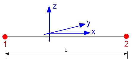
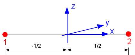
Figure 4.1-a :Reference Item vs Real Item.
The continuous displacement field at any point on the mean line will then be considered in relation to the discretized displacement field in the following manner:
\({U}_{s}=[N].\{U\}\) [éq4.1-1]
Index \(s\) refers to the quantities attached to the average fiber.
Using the shape functions of the reference element, the discretization of variables \({u}_{s}\left(x\right),{v}_{s}\left(x\right),{w}_{s}\left(x\right),{\theta }_{\text{sx}}\left(x\right),{\theta }_{\text{sy}}\left(x\right),{\theta }_{\text{sz}}\left(x\right)\) becomes:
\(\left(\begin{array}{c}{u}_{s}\left(x\right)\\ {v}_{s}\left(x\right)\\ {w}_{s}\left(x\right)\\ {\theta }_{\text{sx}}\left(x\right)\\ {\theta }_{\text{sy}}\left(x\right)\\ {\theta }_{\text{sz}}\left(x\right)\end{array}\right)=\left(\begin{array}{cccccccccccc}{N}_{1}& 0& 0& 0& 0& 0& {N}_{2}& 0& 0& 0& 0& 0\\ 0& {N}_{3}& 0& 0& 0& {N}_{4}& 0& {N}_{5}& 0& 0& 0& {N}_{6}\\ 0& 0& {N}_{3}& 0& -{N}_{4}& 0& 0& 0& {N}_{5}& 0& -{N}_{6}& 0\\ 0& 0& 0& {N}_{1}& 0& 0& 0& 0& 0& {N}_{2}& 0& 0\\ 0& 0& -{N}_{3,x}& 0& {N}_{4,x}& 0& 0& 0& -{N}_{5,x}& 0& {N}_{6,x}& 0\\ 0& {N}_{3,x}& 0& 0& 0& {N}_{4,x}& 0& {N}_{5,x}& 0& 0& 0& {N}_{6,x}\end{array}\right)\cdot \left(\begin{array}{c}{u}_{1}\\ {v}_{1}\\ {w}_{1}\\ {\theta }_{x1}\\ {\theta }_{y1}\\ {\theta }_{z1}\\ {u}_{2}\\ {v}_{2}\\ {w}_{2}\\ {\theta }_{x2}\\ {\theta }_{y2}\\ {\theta }_{z2}\end{array}\right)\)
[éq4.1-2]
With the following interpolation functions, and their useful derivatives:
\(\begin{array}{ccc}{N}_{1}=1-\frac{x}{L}& ;& {N}_{\mathrm{1,}x}=-\frac{1}{L}\\ {N}_{2}=\frac{x}{L}& ;& {N}_{\mathrm{2,}x}=\frac{1}{L}\\ {N}_{3}=1-3\frac{{x}^{2}}{{L}^{2}}+2\frac{{x}^{3}}{{L}^{3}}& ;& {N}_{\mathrm{3,}\mathit{xx}}=-\frac{6}{{L}^{2}}+12\frac{x}{{L}^{3}}\\ {N}_{4}=x-2\frac{{x}^{2}}{L}+\frac{{x}^{3}}{{L}^{2}}& ;& {N}_{\mathrm{4,}\mathit{xx}}=-\frac{4}{L}+6\frac{x}{{L}^{2}}\\ {N}_{5}=3\frac{{x}^{2}}{{L}^{2}}-2\frac{{x}^{3}}{{L}^{3}}& ;& {N}_{\mathrm{5,}\mathit{xx}}=\frac{6}{{L}^{2}}-12\frac{x}{{L}^{3}}\\ {N}_{6}=-\frac{{x}^{2}}{L}+\frac{{x}^{3}}{{L}^{2}}& ;& {N}_{\mathrm{6,}\mathit{xx}}=-\frac{2}{L}+6\frac{x}{{L}^{2}}\end{array}\) [éq4.1-3]
4.2. Determination of the stiffness matrix of the multifiber element#
4.2.1. General case (Euler beam)#
Consider an Euler beam, straight, oriented in the direction \(x\), subjected to distributed forces \({q}_{x},{q}_{y},{q}_{z}\) [Figure].
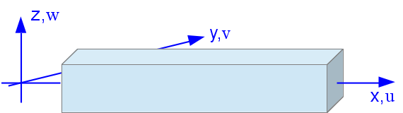
Figure 4.2.1-a : 3D Euler beam.
The displacement and deformation fields then take the following form when writing the displacement of any point in the section as a function of the displacement \(({U}_{s})\) and the rotation \({\theta }_{s}\) of the mean line:
\(u(x,y,z)={u}_{s}(x)-y{\theta }_{\mathit{sz}}(x)+z{\theta }_{\mathit{sy}}(x)\) [éq4.2.1-1]
\(v(x,y,z)={v}_{s}(x)\) [éq4.2.1-2]
\(w(x,y,z)={w}_{s}(x)\) [éq4.2.1-3]
\({\epsilon }_{\mathit{xx}}={u}_{x}^{\text{'}}(x)-y{\theta }_{\mathit{sz}}^{\text{'}}(x)+z{\theta }_{\mathit{sy}}^{\text{'}}(x)\) [éq4.2.1-4]
\({\epsilon }_{\text{xy}}={\epsilon }_{\text{xz}}=0\) [éq4.2.1-5]
Notes:
Torsion is treated globally by assuming an elastic hypothesis, except that we do not calculate \({\epsilon }_{\mathit{yz}}\) here. \(f’(x)\) refers to the derivative of \(f(x)\) with respect to \(x\) .
By introducing the equations [eq] and [eq] into the principle of virtual work we obtain:
\({\int }_{{V}_{0}}{\mathrm{\sigma }}_{\text{xx}}.\mathrm{\delta }{\mathrm{\epsilon }}_{\text{xx}}{\text{dV}}_{0}={\int }_{0}^{L}\left({\mathit{\delta u}}_{s}\left(x\right){q}_{x}+{\mathit{\delta v}}_{s}\left(x\right){q}_{y}+{\mathit{\delta w}}_{s}\left(x\right){q}_{z}\right)\text{dx}\) [éq4.2.1-6]
\({q}_{x},{q}_{y},{q}_{z}\) designating the linear forces applied. This gives using the equation [eq]:
\(\begin{array}{c}{\int }_{0}^{L}\left(N{\mathit{\delta u}}_{s}^{\text{'}}\left(x\right)+{M}_{x}{\mathit{\delta \theta }}_{\text{sx}}^{\text{'}}\left(x\right)+{M}_{y}{\mathit{\delta \theta }}_{\text{sy}}^{\text{'}}\left(x\right)+{M}_{z}{\mathit{\delta \theta }}_{\text{sz}}^{\text{'}}\left(x\right)\right)\text{dx}\\ \hfill \text{=}{\int }_{0}^{L}\left({q}_{x}{\mathit{\delta u}}_{s}\left(x\right)+{q}_{y}{\mathit{\delta v}}_{s}\left(x\right)+{q}_{z}{\mathit{\delta w}}_{s}\left(x\right)\right)\text{dx}\end{array}\) [éq4.2.1-7]
with:
\(N={\int }_{\phantom{\rule{0.5em}{0ex}}S}{\mathrm{\sigma }}_{\text{xx}}\text{dS}\phantom{\rule{2em}{0ex}};\phantom{\rule{2em}{0ex}}{M}_{y}={\int }_{\phantom{\rule{0.5em}{0ex}}S}z{\mathrm{\sigma }}_{\text{xx}}\text{dS}\phantom{\rule{2em}{0ex}};\phantom{\rule{2em}{0ex}}{M}_{z}={\int }_{\phantom{\rule{0.5em}{0ex}}S}-y{\mathrm{\sigma }}_{\text{xx}}\text{dS}\) [éq4.2.1-8]
Notes:
Torsion \({M}_{x}\) is not calculated by integration but calculated directly from the torsional stiffness (see [eq ]) .
The theory of beams associated with an elastic material gives: \({\mathrm{\sigma }}_{\text{xx}}=E{\mathrm{\epsilon }}_{\text{xx}}\)
4.2.2. Case of the multifiber beam#
We now assume that section \(s\) is not homogeneous, materials with different mechanical characteristics.
Without adopting any particular hypothesis about the intersection of axis \(x\) with section \(s\) or about the orientation of the axes \(Y,Z\), the relationship between « generalized » stresses and « generalized » deformations \({\mathrm{D}}_{s}\) becomes [bib2]:
\({\mathrm{F}}_{s}={\mathrm{K}}_{s}\cdot {\mathrm{D}}_{s}\) [éq4.2.2-1]
with:
\(\begin{array}{c}{\mathrm{F}}_{s}={\left(N,\phantom{\rule{0.5em}{0ex}}{M}_{y},\phantom{\rule{0.5em}{0ex}}{M}_{z},\phantom{\rule{0.5em}{0ex}}{M}_{x}\right)}^{T}\\ {\mathrm{D}}_{s}={\left({u}_{s}^{\text{'}}\left(x\right),\phantom{\rule{0.5em}{0ex}}{\theta }_{\text{sy}}^{\text{'}}\left(x\right),\phantom{\rule{0.5em}{0ex}}{\theta }_{\text{sz}}^{\text{'}}\left(x\right),\phantom{\rule{0.5em}{0ex}}{\theta }_{\text{sx}}^{\text{'}}\left(x\right)\right)}^{T}\end{array}\) [éq4.2.2-2]
The matrix \({K}_{s}\) can then be put in the following form:
\({\mathrm{K}}_{s}=\left(\begin{array}{cccc}{K}_{s\text{11}}& {K}_{s\text{12}}& {K}_{s\text{13}}& 0\\ & {K}_{s\text{22}}& {K}_{s\text{23}}& 0\\ & & {K}_{s\text{33}}& 0\\ \text{sym}& & & {K}_{s\text{44}}\end{array}\right)\) [éq4.2.2-3]
with:
\(\begin{array}{c}{K}_{s\text{11}}={\int }_{\phantom{\rule{0.5em}{0ex}}S}\text{EdS}\phantom{\rule{2em}{0ex}};\phantom{\rule{2em}{0ex}}{K}_{s\text{12}}={\int }_{\phantom{\rule{0.5em}{0ex}}S}\text{Ezds}\phantom{\rule{2em}{0ex}};\phantom{\rule{2em}{0ex}}{K}_{s\text{13}}=-{\int }_{\phantom{\rule{0.5em}{0ex}}S}\text{Eyds}\\ {K}_{s\text{22}}={\int }_{\phantom{\rule{0.5em}{0ex}}S}{\text{Ez}}^{2}\text{dS}\phantom{\rule{2em}{0ex}};\phantom{\rule{2em}{0ex}}{K}_{s\text{23}}=-{\int }_{\phantom{\rule{0.5em}{0ex}}S}\text{Eyzds}\phantom{\rule{2em}{0ex}};\phantom{\rule{2em}{0ex}}{K}_{s\text{33}}={\int }_{\phantom{\rule{0.5em}{0ex}}S}{\text{Ey}}^{2}\text{ds}\end{array}\) [éq4.2.2-4]
where \(E\) may vary depending on \(y\) and \(z\). Indeed, it is possible that in the plane modeling of the section, several materials coexist. For example, in a reinforced concrete section, there is both concrete and reinforcement.
The discretization of the fiber section makes it possible to calculate the integrals of the equations [eq]. The calculation of the coefficients of the matrix \({\mathrm{K}}_{s}\) is detailed in the following paragraph [§4.2.3].
Note:
The term of torsion \({K}_{s\text{44}}={\text{GJ}}_{x}\) is given by the user using the data of \({J}_{x}\) , using the command AFFE_CARA_ELEM.
The introduction of the equations [eq] to [eq] in the principle of virtual work leads to:
\({\int }_{\phantom{\rule{0.5em}{0ex}}0}^{\phantom{\rule{0.5em}{0ex}}L}{\mathit{\delta D}}_{s}^{T}\text{.}{K}_{s}\text{.}{D}_{s}\phantom{\rule{0.5em}{0ex}}\text{dx}-{\int }_{\phantom{\rule{0.5em}{0ex}}0}^{\phantom{\rule{0.5em}{0ex}}L}\left({\mathit{\delta u}}_{s}\left(x\right)\phantom{\rule{0.5em}{0ex}}{q}_{x}+{\mathit{\delta v}}_{s}\left(x\right)\phantom{\rule{0.5em}{0ex}}{q}_{y}+{\mathit{\delta w}}_{s}\left(x\right)\phantom{\rule{0.5em}{0ex}}{q}_{z}\right)\phantom{\rule{0.5em}{0ex}}\text{dx}=0\) [éq4.2.2-5]
The generalized deformations are calculated by (\({D}_{S}\) is given to equation [eq]):
\({\mathrm{D}}_{s}=\mathrm{B}\left\{\mathrm{U}\right\}\) [éq4.2.2-6]
With the following \(\mathrm{B}\) matrix:
\(B=\lfloor \begin{array}{cccccccccccc}{N}_{1,x}& 0& 0& 0& 0& 0& {N}_{2,x}& 0& 0& 0& 0& 0\\ 0& 0& -{N}_{\mathrm{3,}\text{xx}}& 0& {N}_{\mathrm{4,}\text{xx}}& 0& 0& 0& -{N}_{\mathrm{5,}\text{xx}}& 0& {N}_{\mathrm{6,}\text{xx}}& 0\\ 0& {N}_{\mathrm{3,}\text{xx}}& 0& 0& 0& {N}_{\mathrm{4,}\text{xx}}& 0& {N}_{\mathrm{5,}\text{xx}}& 0& 0& 0& {N}_{\mathrm{6,}\text{xx}}\\ 0& 0& 0& {N}_{1,x}& 0& 0& 0& 0& 0& {N}_{2,x}& 0& 0\end{array}\rfloor\) [éq4.2.2-7]
Discretizing space \(\left[0,L\right]\) with elements and using equations [eq] makes equation [eq] equivalent to solving a classical linear system:
\(\mathrm{K}\text{.}\mathrm{U}=\mathrm{F}\) [éq4.2.2-8]
The stiffness matrix of the element [Figure] and the vector of the resulting forces are finally given by:
\(\begin{array}{c}{\mathrm{K}}_{\text{elem}}={\int }_{\phantom{\rule{0.5em}{0ex}}0}^{\phantom{\rule{0.5em}{0ex}}L}{\mathrm{B}}^{T}\text{.}{\mathrm{K}}_{s}\text{.}\mathrm{B}\phantom{\rule{1em}{0ex}}\text{dx}\\ \mathrm{F}={\int }_{\phantom{\rule{0.5em}{0ex}}0}^{\phantom{\rule{0.5em}{0ex}}L}{\mathrm{N}}^{T}\text{.}Q\phantom{\rule{1em}{0ex}}\text{dx}\end{array}\) [éq4.2.2-9]
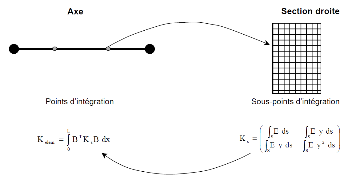
Figure 4.2.2-a : Multifiber beam — Calculation of \({\text{K}}_{\mathit{elem}}\)
With the vector \(Q\) that depends on external loading: \(\mathrm{Q}={\left({q}_{x}\phantom{\rule{1.5em}{0ex}}{q}_{y}\phantom{\rule{1.5em}{0ex}}{q}_{z}\phantom{\rule{1.5em}{0ex}}0\phantom{\rule{1.5em}{0ex}}0\phantom{\rule{1.5em}{0ex}}0\right)}^{T}\).
If we consider that the distributed forces \({q}_{x},{q}_{y},{q}_{z}\) are constant, we get the following nodal forces vector:
\(\mathrm{F}={\left(\frac{{\mathit{Lq}}_{x}}{2}\phantom{\rule{1.5em}{0ex}}\frac{{\mathit{Lq}}_{y}}{2}\phantom{\rule{1.5em}{0ex}}\frac{{\mathit{Lq}}_{z}}{2}\phantom{\rule{1.5em}{0ex}}0\phantom{\rule{1.5em}{0ex}}-\frac{{L}^{2}{q}_{z}}{12}\phantom{\rule{1.5em}{0ex}}\frac{{L}^{2}{q}_{y}}{12}\phantom{\rule{1.5em}{0ex}}\frac{{\mathit{Lq}}_{x}}{2}\phantom{\rule{1.5em}{0ex}}\frac{{\mathit{Lq}}_{y}}{2}\phantom{\rule{1.5em}{0ex}}\frac{{\mathit{Lq}}_{z}}{2}\phantom{\rule{1.5em}{0ex}}0\phantom{\rule{1.5em}{0ex}}\frac{{L}^{2}{q}_{z}}{12}\phantom{\rule{1.5em}{0ex}}\frac{{L}^{2}{q}_{y}}{12}\phantom{\rule{1.5em}{0ex}}\right)}^{T}\) [éq4.2.2-10]
4.2.3. Discretization of the fiber section — Calculation of \({K}_{s}\)#
The discretization of the fiber section makes it possible to calculate the various integrals that are involved in the stiffness matrix, and the other necessary terms.
The geometry of the fibers grouped into fiber groups, via the operator DEFI_GEOM_FIBRE [U4.26.01]) contains in particular the characteristics (Y, Z, AIRE) for each fiber. A maximum of 10 fiber groups can be provided per beam element.
So, if we have a section that has \(n\) fibers we will have the following approximations of the integrals:
\(\begin{array}{c}{K}_{s\text{11}}=\sum _{i=1}^{n}{E}_{i}{S}_{i}\phantom{\rule{2em}{0ex}};\phantom{\rule{2em}{0ex}}{K}_{s\text{12}}=\sum _{i=1}^{n}{E}_{i}{z}_{i}{S}_{i}\phantom{\rule{2em}{0ex}};\phantom{\rule{2em}{0ex}}{K}_{s\text{13}}=\sum _{i=1}^{n}{E}_{i}{y}_{i}{S}_{i}\\ {K}_{s\text{22}}=\sum _{i=1}^{n}{E}_{i}{z}_{{i}^{2}}{S}_{i}\phantom{\rule{2em}{0ex}};\phantom{\rule{2em}{0ex}}{K}_{s\text{23}}=-\sum _{i=1}^{n}{E}_{i}{y}_{i}{z}_{i}{S}_{i}\phantom{\rule{2em}{0ex}};\phantom{\rule{2em}{0ex}}{K}_{s\text{33}}=\sum _{i=1}^{n}{E}_{i}{y}_{{i}^{2}}{S}_{i}\end{array}\) [éq4.2.3-1]
with \({E}_{i}\) the initial or tangent module and \({S}_{i}\) the section of each fiber. The stress state is constant per fiber.
Each fiber is also identified using \({y}_{i}\) and \({z}_{i}\) the coordinates of the fiber’s center of gravity in relation to the axis of the section defined by the keyword “COOR_AXE_POUTRE” (see the command DEFI_GEOM_FIBRE [U4.26.01]).
Fiber numbering depends on the choice of the keyword “FIBRE” or “SECTION” (see command DEFI_GEOM_FIBRE [U4.26.01]).
4.2.4. Integration in the linear elastic case (RIGI_MECA)#
When the behavior of the material is linear, if the beam element is homogeneous in its length, the integration of the equation [eq] can be done analytically.
The following stiffness matrix is then obtained:
\({\mathrm{K}}_{\mathit{elem}}=\left(\begin{array}{cccccccccccc}\frac{{K}_{s\text{11}}}{L}& 0& 0& 0& \frac{{K}_{s\text{12}}}{L}& \frac{{K}_{s\text{13}}}{L}& \frac{-{K}_{s\text{11}}}{L}& 0& 0& 0& \frac{-{K}_{s\text{12}}}{L}& \frac{-{K}_{s\text{13}}}{L}\\ & \frac{\text{12}{K}_{s\text{33}}}{{L}^{3}}& \frac{-\text{12}{K}_{s\text{23}}}{{L}^{3}}& 0& \frac{\text{6}{K}_{s\text{23}}}{{L}^{2}}& \frac{\text{6}{K}_{s\text{33}}}{{L}^{2}}& 0& \frac{-\text{12}{K}_{s\text{33}}}{{L}^{3}}& \frac{\text{12}{K}_{s\text{23}}}{{L}^{3}}& 0& \frac{\text{6}{K}_{s\text{23}}}{{L}^{2}}& \frac{\text{6}{K}_{s\text{33}}}{{L}^{2}}\\ & & \frac{\text{12}{K}_{s\text{22}}}{{L}^{3}}& 0& \frac{-\text{6}{K}_{s\text{22}}}{{L}^{2}}& \frac{-\text{6}{K}_{s\text{23}}}{{L}^{2}}& 0& \frac{\text{12}{K}_{s\text{23}}}{{L}^{3}}& \frac{-\text{12}{K}_{s\text{22}}}{{L}^{3}}& 0& \frac{-\text{6}{K}_{s\text{22}}}{{L}^{2}}& \frac{-\text{6}{K}_{s\text{23}}}{{L}^{2}}\\ & & & \frac{{K}_{s\text{44}}}{L}& 0& 0& 0& 0& 0& -\frac{{K}_{s\text{44}}}{L}& 0& 0\\ & & & & \frac{\text{4}{K}_{s\text{22}}}{L}& \frac{\text{4}{K}_{s\text{23}}}{L}& \frac{-{K}_{s\text{12}}}{L}& \frac{-\text{6}{K}_{s\text{23}}}{{L}^{2}}& \frac{\text{6}{K}_{s\text{22}}}{{L}^{2}}& 0& \frac{\text{2}{K}_{s\text{22}}}{L}& \frac{\text{2}{K}_{s\text{23}}}{L}\\ & & & & & \frac{\text{4}{K}_{s\text{33}}}{L}& \frac{-{K}_{s\text{13}}}{L}& \frac{-\text{6}{K}_{s\text{33}}}{{L}^{2}}& \frac{\text{6}{K}_{s\text{23}}}{{L}^{2}}& 0& \frac{\text{2}{K}_{s\text{23}}}{L}& \frac{\text{2}{K}_{s\text{33}}}{L}\\ & & & & & & \frac{{K}_{s\text{11}}}{L}& 0& 0& 0& \frac{{K}_{s\text{12}}}{L}& \frac{{K}_{s\text{13}}}{L}\\ & & & & & & & \frac{\text{12}{K}_{s\text{33}}}{{L}^{3}}& \frac{-\text{12}{K}_{s\text{23}}}{{L}^{3}}& 0& \frac{-\text{6}{K}_{s\text{23}}}{{L}^{2}}& \frac{-\text{6}{K}_{s\text{33}}}{{L}^{2}}\\ & & & \text{SYM}& & & & & \frac{\text{12}{K}_{s\text{22}}}{{L}^{3}}& 0& \frac{\text{6}{K}_{s\text{22}}}{{L}^{2}}& \frac{6{K}_{s\text{23}}}{{L}^{2}}\\ & & & & & & & & & \frac{{K}_{s\text{44}}}{L}& 0& 0\\ & & & & & & & & & & \frac{\text{4}{K}_{s\text{22}}}{L}& \frac{\text{4}{K}_{s\text{23}}}{L}\\ & & & & & & & & & & & \frac{\text{4}{K}_{s\text{33}}}{L}\end{array}\right)\)
[éq4.2.4-1]
with the following terms \({K}_{s\text{11}},{K}_{s\text{12}},{K}_{s\text{13}},{K}_{s\text{22}},{K}_{s\text{33}},{K}_{s\text{23}},{K}_{s\text{44}}\) given to equation [eq].
Note:
The stiffness matrix presented above does not take into account any eccentricity of the reference axis with respect to the elastic center, in order not to make the presentation heavier. However, additional terms are well taken into account in programming (see §4.5.3).
4.2.5. Integration in the non-linear case (RIGI_MECA_TANG)#
When the behavior of the material is non-linear, to allow a correct integration of internal forces (see paragraph [§4.4]), it is necessary to have at least two integration points along the beam. We chose to use two Gauss points.
The integral of \({\mathrm{K}}_{\mathit{elem}}\) [eq] is calculated in numerical form:
\({\mathrm{K}}_{\mathit{elem}}={\int }_{0}^{L}{\mathrm{B}}^{T}\text{.}{{\rm K}}_{s}\text{.}\mathrm{B}\text{dx}=j\sum _{i=1}^{2}{w}_{i}\mathrm{B}{\left({x}_{i}\right)}^{T}\text{.}{\mathrm{K}}_{s}\left({x}_{i}\right)\text{.}\mathrm{B}\left({x}_{i}\right)\) [éq4.2.5-1]
where \({x}_{i}\) is the position of the Gauss point \(i\) in a reference element of length 1, i.e.: \((1\pm \mathrm{0,57735026918963})/2\);
\({w}_{i}\) is the weight of the \(i\) Gauss point. Here we take \({w}_{i}=\mathrm{0,5}\) for each of the 2 points; \(j\) is the Jacobian. Here we take \(j=L\), the real element having a length \(L\) and the shape function to pass to the reference element being \(\frac{x}{L}\).
\({\mathrm{K}}_{s}\) is calculated using the equations [eq], [eq] (see paragraph [§4.2.3] for the numerical integration of these equations).
The analytical calculation of \(\mathrm{B}{\left({x}_{i}\right)}^{T}\text{.}{\mathrm{K}}_{s}\left({x}_{i}\right)\text{.}\mathrm{B}\left({x}_{i}\right)\) gives:
\(\left(\begin{array}{cccccccccccc}{B}_{1}^{2}{K}_{s\text{11}}& -{B}_{1}{B}_{2}{K}_{s\text{13}}& {B}_{1}{B}_{2}{K}_{s\text{12}}& 0& -{B}_{1}{B}_{3}{K}_{s\text{12}}& -{B}_{1}{B}_{3}{K}_{s\text{13}}& -{B}_{1}^{2}{K}_{s\text{11}}& {B}_{1}{B}_{2}{K}_{s\text{13}}& -{B}_{1}{B}_{2}{K}_{s\text{12}}& 0& -{B}_{1}{B}_{4}{K}_{s\text{12}}& -{B}_{1}{B}_{4}{K}_{s\text{13}}\\ & {B}_{2}^{2}{K}_{s\text{33}}& {B}_{2}^{2}{K}_{s\text{23}}& 0& {B}_{2}{B}_{3}{K}_{s\text{23}}& {B}_{2}{B}_{3}{K}_{s\text{33}}& {B}_{1}{B}_{2}{K}_{s\text{13}}& -{B}_{2}^{2}{K}_{s\text{33}}& {B}_{2}^{2}{K}_{s\text{23}}& 0& {B}_{2}{B}_{4}{K}_{s\text{23}}& {B}_{2}{B}_{4}{K}_{s\text{33}}\\ & & {B}_{2}^{2}{K}_{s\text{22}}& 0& -{B}_{2}{B}_{3}{K}_{s\text{22}}& -{B}_{2}{B}_{3}{K}_{s\text{23}}& -{B}_{1}{B}_{2}{K}_{s\text{12}}& {B}_{2}^{2}{K}_{s\text{23}}& -{B}_{2}^{2}{K}_{s\text{22}}& 0& -{B}_{2}{B}_{4}{K}_{s\text{22}}& -{B}_{2}{B}_{4}{K}_{s\text{23}}\\ & & & {B}_{1}^{2}{K}_{s\text{44}}& 0& 0& 0& 0& 0& -{B}_{1}^{2}{K}_{s\text{44}}& 0& 0\\ & & & & {B}_{3}^{2}{K}_{s\text{22}}& {B}_{3}^{2}{K}_{s\text{23}}& {B}_{1}{B}_{3}{K}_{s\text{12}}& -{B}_{2}{B}_{3}{K}_{s\text{23}}& {B}_{2}{B}_{3}{K}_{s\text{22}}& 0& {B}_{3}{B}_{4}{K}_{s\text{22}}& {B}_{3}{B}_{4}{K}_{s\text{23}}\\ & & & & & {B}_{3}^{2}{K}_{s\text{33}}& {B}_{1}{B}_{3}{K}_{s\text{13}}& -{B}_{2}{B}_{3}{K}_{s\text{33}}& {B}_{2}{B}_{3}{K}_{s\text{23}}& 0& {B}_{3}{B}_{4}{K}_{s\text{23}}& {B}_{3}{B}_{4}{K}_{s\text{33}}\\ & & & & & & {B}_{1}^{2}{K}_{s\text{11}}& -{B}_{1}{B}_{2}{K}_{s\text{13}}& {B}_{1}{B}_{2}{K}_{s\text{12}}& 0& {B}_{1}{B}_{4}{K}_{s\text{12}}& {B}_{1}{B}_{4}{K}_{s\text{13}}\\ & & & & & & & {B}_{2}^{2}{K}_{s\text{33}}& -{B}_{2}^{2}{K}_{s\text{23}}& 0& -{B}_{2}{B}_{4}{K}_{s\text{23}}& -{B}_{2}{B}_{4}{K}_{s\text{33}}\\ & & & & & & & & {B}_{2}^{2}{K}_{s\text{22}}& 0& {B}_{2}{B}_{4}{K}_{s\text{22}}& {B}_{2}{B}_{4}{K}_{s\text{23}}\\ & & & & & & & & & {B}_{1}^{2}{K}_{s\text{44}}& 0& 0\\ & & & & & & & & & & {B}_{4}^{2}{K}_{s\text{22}}& {B}_{4}^{2}{K}_{s\text{23}}\\ & & & & & & & & & & & {B}_{4}^{2}{K}_{s\text{33}}\end{array}\right)\) [éq4.2.5-2]
where \({B}_{i}\) are calculated at the \({x}_{i}\) coordinate of the reference element with:
\(\begin{array}{c}{B}_{1}=-{N}_{\mathrm{1,}x}={N}_{\mathrm{2,}x}=\frac{1}{L}\\ {B}_{2}=-{N}_{\mathrm{3,}\mathit{xx}}={N}_{\mathrm{5,}\mathit{xx}}=-\frac{6}{{L}^{2}}+\frac{12{x}_{i}}{{L}^{2}}\\ {B}_{3}={N}_{\mathrm{4,}\mathit{xx}}=-\frac{4}{L}+\frac{6{x}_{i}}{L}\\ {B}_{4}={N}_{\mathrm{6,}\mathit{xx}}=-\frac{2}{L}+\frac{6{x}_{i}}{L}\end{array}\) [éq4.2.5-3]
4.3. Determination of the mass matrix of the multifiber element#
4.3.1. Determining \({\mathrm{M}}_{\mathit{elem}}\)#
Likewise, the virtual work of inertial efforts becomes [bib2]:
\(\begin{array}{c}{W}_{\text{inert}}={\int }_{0}^{L}{\int }_{S}\rho \left(\mathit{\delta u}\left(x,y\right)\frac{{d}^{2}u\left(x,y\right)}{{\text{dt}}^{2}}+\mathit{\delta v}\left(x,y\right)\frac{{d}^{2}v\left(x,y\right)}{{\text{dt}}^{2}}+\mathit{\delta w}\left(x,y\right)\frac{{d}^{2}w\left(x,y\right)}{{\text{dt}}^{2}}\right)\text{dS}\text{dx}\\ ={\int }_{0}^{L}\delta {\mathrm{U}}_{s}\text{.}{\mathrm{M}}_{s}\text{.}\frac{{d}^{2}{\mathrm{U}}_{s}}{{\text{dt}}^{2}}\text{dx}\end{array}\) [éq4.3.1-1]
with \({\mathrm{U}}_{s}\) the vector of « generalized » movements.
This gives for the mass matrix:
\({\mathrm{M}}_{s}=\left(\begin{array}{cccccc}{M}_{s\text{11}}& 0& 0& 0& {M}_{s\text{12}}& {M}_{s\text{13}}\\ & {M}_{s\text{11}}& 0& -{M}_{s\text{12}}& 0& 0\\ & & {M}_{s\text{11}}& -{M}_{s\text{13}}& 0& 0\\ & & & {M}_{s\text{22}}+{M}_{s\text{33}}& 0& 0\\ & & & & {M}_{s\text{22}}& {M}_{s\text{23}}\\ \text{sym}& & & & & {M}_{s\text{33}}\end{array}\right)\) [éq4.3.1-2]
with:
\(\begin{array}{c}{M}_{s\text{11}}={\int }_{S}\rho \text{ds};{M}_{s\text{12}}={\int }_{S}\rho \text{zds};{M}_{s\text{13}}=-{\int }_{S}\rho \text{yds}\\ {M}_{s\text{22}}={\int }_{S}\rho {z}^{2}\text{ds};{M}_{s\text{23}}=-{\int }_{S}\rho \text{yzds};{M}_{s\text{33}}={\int }_{S}\rho {y}^{2}\text{ds}\end{array}\) [éq4.3.1-3]
with \(\rho\) which may vary depending on \(y\) and \(z\).
As for the stiffness matrix, we take into account the generalized deformations and the discretization of space \(\left[\mathrm{0,}L\right]\). This finally gives for the elementary mass matrix of dimension \(\mathrm{12x12}\):
\({M}_{\mathit{elem}}^{1}=\left[\frac{{\mathit{LM}}_{s\text{11}}}{3}\frac{-{M}_{s\text{13}}}{2}\frac{{M}_{s\text{12}}}{2}0\frac{{\mathit{LM}}_{s\text{12}}}{12}\frac{{\mathit{LM}}_{s\text{13}}}{12}\frac{{\mathit{LM}}_{s\text{11}}}{6}\frac{{M}_{s\text{13}}}{2}\frac{-{M}_{s\text{12}}}{2}0\frac{-L{M}_{s\text{12}}}{12}\frac{-L{M}_{s\text{13}}}{12}\right]\)
\({M}_{\mathit{elem}}^{2}=\left[\mathit{sym}\frac{\text{13}L{M}_{s\text{11}}}{35}+\frac{\text{6}{M}_{s\text{33}}}{5L}\frac{-\text{6}{M}_{s\text{23}}}{5L}\frac{-\text{7}{\mathit{LM}}_{s\text{12}}}{20}\frac{{M}_{s\text{23}}}{10}\frac{\text{11}{L}^{2}{M}_{s\text{11}}}{210}+\frac{{M}_{s\text{33}}}{10}\frac{-{M}_{s\text{13}}}{2}\frac{\text{9}{\mathit{LM}}_{s\text{11}}}{70}-\frac{\text{6}{M}_{s\text{33}}}{5L}\frac{\text{6}{M}_{s\text{23}}}{5L}\frac{-\mathrm{3L}{M}_{s\text{12}}}{20}\frac{{M}_{s\text{23}}}{10}\frac{-\text{13}{L}^{2}{M}_{s\text{11}}}{420}+\frac{{M}_{s\text{33}}}{10}\right]\)
\({M}_{\mathit{elem}}^{3}=\left[\mathit{sym}\mathit{sym}\frac{\text{13}{\mathit{LM}}_{s\text{11}}}{35}+\frac{\text{6}{M}_{s\text{22}}}{5L}\frac{-\text{7}L{M}_{s\text{13}}}{20}\frac{-\text{11}{L}^{2}{M}_{s\text{11}}}{210}-\frac{{M}_{s\text{22}}}{10}\frac{-{M}_{s\text{23}}}{10}\frac{{M}_{s\text{12}}}{2}\frac{\text{6}{M}_{s\text{23}}}{5L}\frac{\text{9}{\mathit{LM}}_{s\text{11}}}{70}-\frac{\text{6}{M}_{s\text{22}}}{5L}\frac{-{\mathrm{3LM}}_{s\text{13}}}{20}\frac{\text{13}{L}^{2}{M}_{s\text{11}}}{420}-\frac{{M}_{s\text{22}}}{10}\frac{-{M}_{s\text{23}}}{10}\right]\)
\({M}_{\mathit{elem}}^{4}=\left[\mathit{sym}\mathit{sym}\mathit{sym}\frac{{\mathit{LM}}_{s\text{22}}+{\mathit{LM}}_{s\text{33}}}{3}\frac{{L}^{2}{M}_{s\text{13}}}{20}\frac{-{L}^{2}{M}_{s\text{12}}}{20}0\frac{-{\mathrm{3LM}}_{s\text{12}}}{20}\frac{-\mathrm{3L}{M}_{s\text{13}}}{20}\frac{{\mathit{LM}}_{s\text{22}}+L{M}_{s\text{33}}}{6}\frac{-{L}^{2}{M}_{s\text{13}}}{30}\frac{{L}^{2}{M}_{s\text{12}}}{30}\right]\)
\({M}_{\mathit{elem}}^{5}=\left[\mathit{sym}\mathit{sym}\mathit{sym}\mathit{sym}\frac{{L}^{3}{M}_{s\text{11}}}{105}+\frac{\text{2}{\mathit{LM}}_{s\text{22}}}{15}\frac{\text{2}{\mathit{LM}}_{s\text{23}}}{15}\frac{-{\mathit{LM}}_{s\text{12}}}{12}\frac{-{M}_{s\text{23}}}{10}\frac{-\text{13}{L}^{2}{M}_{s\text{11}}}{420}+\frac{{M}_{s\text{22}}}{10}\frac{{L}^{2}{M}_{s\text{13}}}{30}\frac{-{L}^{3}{M}_{s\text{11}}}{140}-\frac{{\mathit{LM}}_{s\text{22}}}{30}\frac{-{\mathit{LM}}_{s\text{23}}}{30}\right]\)
\({M}_{\mathit{elem}}^{6}=\left[\mathit{sym}\mathit{sym}\mathit{sym}\mathit{sym}\mathit{sym}\frac{{L}^{3}{M}_{s\text{11}}}{105}+\frac{\text{2}{\mathit{LM}}_{s\text{33}}}{15}\frac{-{\mathit{LM}}_{s\text{13}}}{12}\frac{\text{13}{L}^{2}{M}_{s\text{11}}}{420}-\frac{{M}_{s\text{33}}}{10}\frac{{M}_{s\text{23}}}{10}\frac{-{L}^{2}{M}_{s\text{12}}}{30}\frac{-{\mathit{LM}}_{s\text{23}}}{30}\frac{-{L}^{3}{M}_{s\text{11}}}{140}-\frac{{\mathit{LM}}_{s\text{33}}}{30}\right]\)
\({M}_{\mathit{elem}}^{7}=\left[\mathit{sym}\mathit{sym}\mathit{sym}\mathit{sym}\mathit{sym}\mathit{sym}\frac{L{M}_{s\text{11}}}{3}\frac{{M}_{s\text{13}}}{2}\frac{-{M}_{s\text{12}}}{2}0\frac{{\mathit{LM}}_{s\text{12}}}{12}\frac{{\mathit{LM}}_{s\text{13}}}{12}\right]\)
\({M}_{\mathit{elem}}^{8}=\left[\mathit{sym}\mathit{sym}\mathit{sym}\mathit{sym}\mathit{sym}\mathit{sym}\mathit{sym}\frac{\text{13}{\mathit{LM}}_{s\text{11}}}{35}+\frac{\text{6}{M}_{s\text{33}}}{5L}\frac{-\text{6}{M}_{s\text{23}}}{5L}\frac{-\text{7}L{M}_{s\text{12}}}{20}\frac{-{M}_{s\text{23}}}{10}\frac{-\text{11}{L}^{2}{M}_{s\text{11}}}{210}-\frac{{M}_{s\text{33}}}{10}\right]\)
\({M}_{\mathit{elem}}^{9}=\left[\mathit{sym}\mathit{sym}\mathit{sym}\mathit{sym}\mathit{sym}\mathit{sym}\mathit{sym}\mathit{sym}\frac{\text{13}L{M}_{s\text{11}}}{35}+\frac{\text{6}{M}_{s\text{22}}}{5L}\frac{-\text{7}L{M}_{s\text{13}}}{20}\frac{\text{11}{L}^{2}{M}_{s\text{11}}}{210}+\frac{{M}_{s\text{22}}}{10}\frac{{M}_{s\text{23}}}{10}\right]\)
\({M}_{\mathit{elem}}^{10}=\left[\mathit{sym}\mathit{sym}\mathit{sym}\mathit{sym}\mathit{sym}\mathit{sym}\mathit{sym}\mathit{sym}\mathit{sym}\frac{{\mathit{LM}}_{s\text{22}}+{\mathit{LM}}_{s\text{33}}}{3}\frac{-{L}^{2}{M}_{s\text{13}}}{20}\frac{{L}^{2}{M}_{s\text{12}}}{20}\right]\)
\({M}_{\mathit{elem}}^{11}=\left[\mathit{sym}\mathit{sym}\mathit{sym}\mathit{sym}\mathit{sym}\mathit{sym}\mathit{sym}\mathit{sym}\mathit{sym}\mathit{sym}\frac{{L}^{3}{M}_{s\text{11}}}{105}+\frac{\text{2}{\mathit{LM}}_{s\text{22}}}{15}\frac{\text{2}{\mathit{LM}}_{s\text{23}}}{15}\right]\)
\({M}_{\mathit{elem}}^{12}=\left[\mathit{sym}\mathit{sym}\mathit{sym}\mathit{sym}\mathit{sym}\mathit{sym}\mathit{sym}\mathit{sym}\mathit{sym}\mathit{sym}\mathit{sym}\frac{{L}^{3}{M}_{s\text{11}}}{105}+\frac{\text{2}{\mathit{LM}}_{s\text{33}}}{15}\right]\)
with the following terms: \({M}_{s11},{M}_{s12},{M}_{s13},{M}_{s22},{M}_{s33},{M}_{s23}\) that are given to equation [eq].
Notes:
The diagonal mass matrix is reduced by the concentrated mass technique [R3.08.01]. This diagonal mass matrix is obtained by the option “ MASS_MECA_DIAG “from the operator * CALC_MATR_ELEM [U4.61.01].
The additional terms in case of eccentricity of the axes are not presented here but are taken into account (see §4.5.3) .
4.3.2. Discretization of the fiber section - Calculation of \({M}_{s}\)#
The discretization of the fiber section makes it possible to calculate the various integrals that are involved in the mass matrix. So, if we have a section that has \(n\) fibers we will have the following approximations of the integrals:
\(\begin{array}{c}{M}_{s\text{11}}=\sum _{i=1}^{n}{\rho }_{i}{S}_{i};{M}_{s\text{12}}=\sum _{i=1}^{n}{\rho }_{i}{z}_{i}{S}_{i};{M}_{s\text{13}}=-\sum _{i=1}^{n}{\rho }_{i}{y}_{i}{S}_{i}\\ {M}_{s\text{22}}=\sum _{i=1}^{n}{\rho }_{i}{z}_{{i}^{2}}{S}_{i};{M}_{s\text{23}}=-\sum _{i=1}^{n}{\rho }_{i}{y}_{i}{z}_{i}{S}_{i};{M}_{s\text{33}}=\sum _{i=1}^{n}{\rho }_{i}{y}_{{i}^{2}}{S}_{i}\end{array}\) [éq4.3.2-1]
with \({\rho }_{i}\) and \({S}_{i}\) the density and cross section of each fiber. \({y}_{i}\) and \({z}_{i}\) are the coordinates of the fiber’s center of gravity defined as above.
4.4. Calculation of internal forces#
The calculation of nodal forces \({\mathrm{F}}_{\text{int}}\) due to a state of given internal constraints is done by the integral:
\({F}_{\text{int}}={\int }_{0}^{L}{B}^{T}\text{.}{F}_{s}\text{dx}\) [éq4.4-1]
where \(B\) is the matrix giving the generalized deformations as a function of the nodal displacements [eq] and where \({\mathrm{F}}_{\text{s}}\) is the vector of the generalized stresses given to the equation [eq],
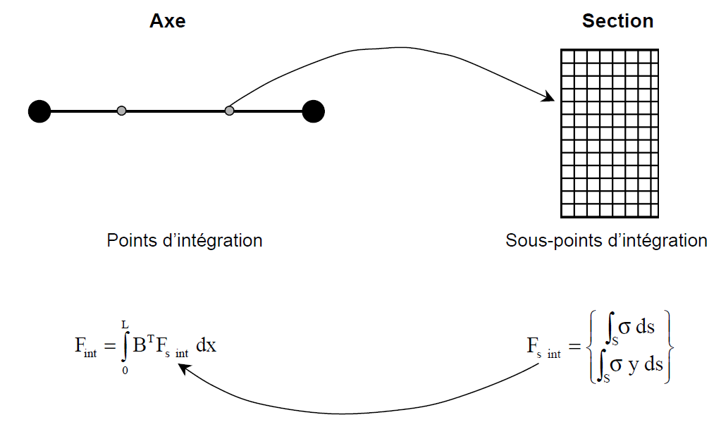
Figure 4.4-a :Multifiber Beam — Calculation of \({\mathrm{F}}_{\text{int}}\)
\({\mathrm{F}}_{s}^{T}=\left(N{M}_{y}{M}_{z}{M}_{x}\right)\) [éq4.4-2]
The normal force N and the bending moments \({M}_{y}\) and \({M}_{z}\) are calculated by integrating the stresses on the section [eq].
Since the torsional behavior is assumed to remain linear, the torsional moment is calculated with the nodal axial rotations:
\({M}_{x}={\mathit{GJ}}_{x}\frac{{\theta }_{x2}-{\theta }_{x1}}{L}\) [éq4.4-3]
The equation [eq] is numerically integrated:
\({\mathrm{F}}_{i}={\int }_{0}^{L}{\mathrm{B}}^{T}\text{.}{\mathrm{F}}_{s}\text{dx}=j\sum _{i=1}^{2}{w}_{i}\mathrm{B}{\left({x}_{i}\right)}^{T}\text{.}{\mathrm{F}}_{s}\left({x}_{i}\right)\) [éq4.4-4]
The positions and weights of the Gauss points as well as the Jacobian are given in paragraph [§4.2.5].
The analytical calculation of \(B{\left({x}_{i}\right)}^{T}\text{.}{F}_{s}\left({x}_{i}\right)\) gives:
\({\left[B{\left({x}_{i}\right)}^{T}\text{.}{F}_{s}\left({x}_{i}\right)\right]}^{T}=\begin{array}{c}[-{B}_{1}N{B}_{2}{M}_{z}-{B}_{2}{M}_{y}0{B}_{3}{M}_{y}{B}_{3}{M}_{z}\\ {B}_{1}N-{B}_{2}{M}_{z}{B}_{2}{M}_{y}0{B}_{4}{M}_{y}{B}_{4}{M}_{z}]\end{array}\) [éq4.4-5]
where \({B}_{i}\) are given to equation [eq].
4.5. Formulation enriched with deformation#
With the displacement interpolations of equation [eq], the generalized axial deformation is constant and the curvatures are linear (see equations [eq], [eq] and [eq]):
\(\{\begin{array}{c}{\epsilon }_{s}(x)=\frac{{u}_{2}-{u}_{1}}{L}\\ {\chi }_{\text{ys}}(x)=-\left(-\frac{6}{{L}^{2}}+\frac{\text{12}x}{{L}^{3}}\right){w}_{1}+\left(\frac{\mathrm{6x}}{{L}^{2}}-\frac{4}{L}\right){\theta }_{\mathit{y1}}-\left(-\frac{\text{12}x}{{L}^{3}}+\frac{6}{{L}^{2}}\right){w}_{2}+\left(\frac{\mathrm{6x}}{{L}^{2}}-\frac{4}{L}\right){\theta }_{\mathit{y2}}\\ {\chi }_{\text{zs}}(x)=\left(-\frac{6}{{L}^{2}}+\frac{\text{12}x}{{L}^{3}}\right){v}_{1}+\left(\frac{\mathrm{6x}}{{L}^{2}}-\frac{4}{L}\right){\theta }_{\mathit{z1}}+\left(-\frac{\text{12}x}{{L}^{3}}+\frac{6}{{L}^{2}}\right){v}_{2}+\left(\frac{\mathrm{6x}}{{L}^{2}}-\frac{4}{L}\right){\theta }_{\mathit{z2}}\end{array}\) [éq4.5-1]
If there is no coupling between these two deformations (elastic case, with the mean reference line that passes through the barycenter of the section), this does not pose problems. But in the general non-linear case, there is a neutral axis shift, and the terms \({K}_{s\text{12}}\) and \({K}_{s\text{13}}\) of \({\mathrm{K}}_{s}\) (equations [eq] and [eq]) are not zero, there is a coupling between the moments and the normal effort. There is then an incompatibility in the approximation of the axial deformations of a fiber:
\(\epsilon ={\epsilon }_{s}(x)-y{\chi }_{\text{zs}}(x)+z{\chi }_{\text{ys}}(x)\) [éq4.5-2]
One way to eliminate this incompatibility is to enrich the axial deformation field:
\({\epsilon }_{s}(x)\mapsto {\epsilon }_{s}(x)+\stackrel{̃}{{\epsilon }_{s}}(x);\stackrel{̃}{{\epsilon }_{s}}(x)=\alpha .G(x);G(x)=\frac{4}{L}-\frac{8x}{{L}^{2}}\) [éq4.5-3]
For \(x\in \left[-\frac{L}{2},\frac{L}{2}\right]\)
where \(G(x)\) is an enriched deformation that derives from a moving « bubble » function and \(\alpha\) is the enrichment degree of freedom. The variational basis for such enrichment is provided by the Hu-Washizu principle [bib5] which can be presented in the same way as the method of incompatible modes [bib6].
4.5.1. Incompatible modes method#
The regular generalized displacement field \({\mathrm{U}}_{s}\) is defined by the equation [eq]. The generalized deformations \({\mathrm{D}}_{s}\) and the generalized stresses \({\mathrm{F}}_{s}\) by the equation [eq].
The Hu-Washizu principle consists in writing the weak form of the equilibrium equations, but also of the calculation of deformations and the law of behavior, in projection onto the three virtual fields (generalized displacements \({\mathrm{U}}_{s}^{\text{*}}\), generalized deformations, generalized deformations \({\mathrm{D}}_{s}^{\text{*}}\), and generalized constraints and generalized constraints \({\mathrm{F}}_{s}^{\text{*}}\)):
\(\{\begin{array}{c}{\int }_{0}^{L}\frac{{\mathit{dU}}_{s}^{\text{*}}}{\text{dx}}\cdot {F}_{s}\text{dx}-{W}_{\text{ext}}=0\\ {\int }_{0}^{L}{F}_{s}^{\text{*}}\cdot \left(\frac{d{U}_{s}}{\text{dx}}-{D}_{s}\right)\text{dx}=0\\ {\int }_{0}^{L}{D}_{s}^{\text{*}}\cdot \left({F}_{s}-{K}_{s}\cdot {D}_{s}\right)\text{dx}=0\end{array}\) [éq4.5.1-1]
The enrichment of real deformations is introduced, and it is chosen to decompose the virtual field of deformations into a « regular » part resulting from the virtual field of movements and an enriched part:
\({D}_{s}=\frac{{\mathit{dU}}_{s}}{\text{dx}}+{\stackrel{̄}{D}}_{s}\) \({D}_{s}^{\text{*}}=\frac{{\mathit{dU}}_{s}^{\text{*}}}{\text{dx}}+{\stackrel{̄}{D}}_{s}^{\text{*}}\) [éq4.5.1-2]
We carry [eqa] into [eqb], which justifies the « enrichment » by orthogonality:
\({\int }_{0}^{L}{\mathrm{F}}_{s}^{\text{*}}\text{.}{\mathrm{D}}_{s}\mathit{dx}=0\) [éq4.5.1-3]
The equation [eqc] is divided into two since we have two independent virtual fields in [eqb]:
\({\int }_{0}^{L}\frac{{\mathit{dU}}_{s}^{\text{*}}}{\text{dx}}\text{.}\left({F}_{s}-{K}_{s}\text{.}{D}_{s}\right)\text{dx}=0\) \({\int }_{0}^{L}{\overline{\text{D}}}_{s}^{\text{*}}\cdot \left({\text{F}}_{s}-{\text{K}}_{s}\cdot {\text{D}}_{s}\right)\mathit{dx}=0\) [éq4.5.1-4]
Finally, the method of incompatible modes consists in choosing the space of the constraints orthogonal to the space of the enriched deformations, in such a way that [eq] is automatically verified and [eqb] therefore simply gives:
\({\int }_{0}^{L}{\stackrel{̄}{\mathrm{D}}}_{s}^{\text{*}}\text{.}{\mathrm{K}}_{s}\text{.}{\mathrm{D}}_{s}\mathit{dx}=0\) [éq4.5.1-5]
If we go back to the strong formulation of the law of behavior in [eqa] and [eq], the system [eq] becomes:
\({\int }_{0}^{L}\frac{{\mathit{dU}}_{s}^{\text{*}}}{\text{dx}}\text{.}{F}_{s}\text{dx}-{W}_{\text{ext}}=0\) \({\int }_{0}^{L}{{\overline{\text{D}}}_{s}}^{\text{*}}\cdot {\text{F}}_{s}\mathit{dx}=0\) \({\text{F}}_{s}={\text{K}}_{s}\cdot {\text{D}}_{s}\) [éq4.5.1-6]
Note:
Here we only enrich the axial deformation of an Euler-Bernoulli beam element, with a continuous function, so \(\stackrel{̄}{\mathrm{D}}={\left(\begin{array}{cccc}\stackrel{̄}{{\epsilon }_{s}}& 0& 0& 0\end{array}\right)}^{T}\).
4.5.2. Digital implementation#
From the point of view of finite elements, we can write the displacements and the deformations in matrix form, with the enriched part:
\({\mathrm{B}}_{s}=\mathrm{N}.(\mathrm{U})+\mathrm{Q}.(\alpha )\) \(\mathrm{D}=\mathrm{B}.(\mathrm{U})+\mathrm{G}.(\alpha )\) [éq4.5.2-1]
where \(\mathrm{N}\) and \(\mathrm{B}\) are the classical matrices of interpolation functions and their derivatives (see [eq] and [eq]) and:
\(\mathrm{Q}={\left(\begin{array}{cccc}\frac{4x}{L}-\frac{4{x}^{2}}{{L}^{2}}& 0& 0& 0\end{array}\right)}^{T}\) and \(\mathrm{G}={\left(\begin{array}{cccc}\frac{4}{L}-\frac{8x}{{L}^{2}}& 0& 0& 0\end{array}\right)}^{T}\) [éq4.5.2-2]
Note:
\(\mathrm{G}\) was chosen so that the element always passes the « patch test » (zero deformation energy for solid motion): \({\int }_{0}^{L}\mathrm{G}(x)\text{dx}=0\) [éq4.5.2-3]
After classical manipulations of transition from continuous to discrete, the system of equations [eq], written for the whole structure, is approximated by:
\(\{\begin{array}{c}{A}_{e=1}^{{N}_{\text{elem}}}\left({F}_{\text{int}}-{F}_{\text{ext}}\right)=0\\ {h}_{e}=0\text{}\forall e\in [\mathrm{1,}{N}_{\text{elem}}]\end{array}\) [éq4.5.2-4]
with:
\(\{\begin{array}{c}{\mathrm{F}}_{\text{int}}={\int }_{0}^{L}{\mathrm{B}}^{T}\text{.}{\mathrm{F}}_{s}\text{dx}={\int }_{0}^{L}{\mathrm{B}}^{T}\text{.}{\mathrm{K}}_{s}\text{.}\left(\mathrm{B}\text{.}{\mathrm{U}}_{s}+\mathrm{G}\text{.}\alpha \right)\text{dx}\\ {\mathrm{F}}_{\text{ext}}={\int }_{0}^{L}{\mathrm{N}}^{T}\text{.}\mathrm{f}\text{dx}\\ {h}_{e}={\int }_{0}^{L}{\mathrm{G}}^{T}\text{.}{\mathrm{F}}_{s}\text{dx}\end{array}\) [éq4.5.2-5]
\({A}_{e=1}^{{N}_{\text{elem}}}\) denotes the assembly across all elements of the mesh; \(\mathrm{f}\) is the axial load distributed over the beam element. The system of equations [eq] is non-linear, it is solved iteratively (see STAT_NON_LINE).
At iteration \((i+1)\), with \(\Delta {\mathrm{U}}^{(i)}={\mathrm{U}}^{(i+1)}-{\mathrm{U}}^{(i)}\) and \(\Delta {\alpha }^{(i)}={\alpha }^{(i+1)}-{\alpha }^{(i)}\), the linearization of the system gives (Newton correction iterations):
\(\{\begin{array}{c}{A}_{e=1}^{{N}_{\text{elem}}}\left(\left({\mathrm{F}}_{\text{int}}^{(i+1)}-{\mathrm{F}}_{\text{ext}}^{(i+1)}\right)+{\mathrm{K}}_{e}^{(i)}.\Delta {\mathrm{U}}^{(i)}+{\mathrm{X}}_{e}^{(i)}\Delta {\alpha }^{(i)}\right)=0\\ {h}_{e}^{(i+1)}+{\mathrm{X}}_{e}^{(i)T}.\Delta {\mathrm{U}}^{(i)}+{H}_{e}^{(i)}\Delta {\alpha }^{(i)}=0\forall e\in [\mathrm{1,.}\mathrm{..},{N}_{\text{elem}}]\end{array}\) [éq4.5.2-6]
with:
\(\{\begin{array}{c}{\mathrm{K}}_{e}^{(i)}={\int }_{L}{\mathrm{B}}^{T}\text{.}{\mathrm{K}}_{s}^{(i)}\text{.}\mathrm{B}\text{dx}\\ {\mathrm{X}}_{e}^{(i)}={\int }_{L}{\mathrm{B}}^{T}\text{.}{\mathrm{K}}_{s}^{(i)}\text{.}\mathrm{G}\text{dx}\\ {H}_{e}^{(i)}={\int }_{L}{\mathrm{G}}^{T}\text{.}{\mathrm{K}}_{s}^{(i)}\text{.}\mathrm{G}\text{dx}\end{array}\) [éq4.5.2-7]
The second equation of the system [eq] is local. It allows you to calculate the degree of freedom of enrichment \(\alpha\) independently on each element. It is calculated by a local iterative method (iterations \((j)\) for a fixed \({d}^{(i)}=\Delta {\mathrm{U}}^{(i)}\) displacement):
\({\alpha }_{(j+1)}^{(i)}={\alpha }_{(j)}^{(i)}-{\left({H}_{e(j)}^{(i)}\right)}^{-1}{h}_{e(j)}^{(i)}\) [éq4.5.2-8]
So, when we converged at the local level, we have:
\({h}_{e}({d}^{(i)},{\alpha }^{(i)})=0\) [éq4.5.2-9]
And static condensation can be performed to eliminate \(\alpha\) globally.
\({\mathrm{K}}_{e}^{(i)}={\mathrm{K}}_{e}^{(i)}-{\mathrm{X}}_{e}^{(i)}{\left({H}_{e}^{(i)}\right)}^{-1}{\mathrm{X}}_{e}^{(i)T}\) [éq4.5.2-10]
From a practical point of view, this technique makes it possible to deal with enrichment at the elementary level without disturbing the number of global degrees of freedom. It is implemented at the level of the elementary routine responsible for calculating the options FULL_MECA, RAPH_MECA and RIGI_MECA_TANG.
Notes:
in the particular case shown here, \({H}_{e}^{(i)}\) is a real one, so very easy to reverse.
similarly, \({h}_{e}\) and \(\alpha\) are also real.
The calculation of \({K}_{e}^{(i)}\) is explained in paragraph §4.2.5, the other quantities of the equation [eq] are calculated using the same technique.
Likewise, the calculation of \({\mathrm{F}}_{\text{int}}\) is explained in paragraph § 4.4, \({h}_{e}\) in the equation [eq] is calculated using the same technique.
4.5.3. Taking into account eccentricity#
For elastic behavior, the enrichment of axial deformations makes it possible to correctly take into account the coupling between the normal force and the bending moments, and to make the response of the beam independent of the position chosen for the reference axis (see keyword COOR_AXE_POUTRE in the operator DEFI_GEOM_FIBRE, [U4.26.01]). It thus makes it possible to treat the case of eccentric beams.
The numerical implementation of the enrichment of axial deformations presented in paragraph 4.5.2 concerns nonlinear calculations with STAT_NON_LINE or DYNA_NON_LINE, for the options FULL_MECA, RAPH_MECA and RIGI_MECA_TANG. Indeed, the determination of \(\alpha\) is done by local iterations at the elementary level [eq].
In the case of calculations with option RIGI_MECA (MECA_STATIQUE, mode calculation, nonlinear calculations with prediction “ELASTIQUE”), it is possible to determine \(\alpha\) explicitly according to the eccentricities of the elastic center with respect to the reference axis:
\({e}_{y}=\frac{{\int }_{S}\mathit{Ey}\mathit{dS}}{{\int }_{S}E\mathit{dS}}=\frac{{K}_{\mathit{S13}}}{{K}_{\mathit{S11}}}\) and \({e}_{z}=\frac{{\int }_{S}\mathit{Ez}\mathit{dS}}{{\int }_{S}E\mathit{dS}}=\frac{{K}_{\mathit{S12}}}{{K}_{\mathit{S11}}}\)
The static condensation can then be treated to eliminate \(\alpha\) at the level of the elementary stiffness matrix. These calculations were done analytically and the matrix is explicitly implemented in*Code_Aster* (modification of about twenty terms if \({e}_{y}\) and/or \({e}_{z}\) are not zero).
Since the displacement is enriched, the mass matrix (see §4.3) is changed. As for the stiffness matrix, the terms modified in the case where \({e}_{y}\) and/or \({e}_{z}\) are not zero, have been calculated analytically and programmed explicitly.
Enriching the deformations also changes the calculation of options DEGE_ELNO [eq] and EPSI_ELGA [eq].
4.6. Usable nonlinear behavior models#
The supported models are on the one hand the 1D behavior relationships of the type VMIS_ISOT_LINE, VMIS_CINE_LINE,,, VMIS_ISOT_TRAC, CORR_ACIER and PINTO_MENEGOTTO [R5.03.09] for steels, on the other hand the model MAZARS_UNIL [R7.01.08] dedicated to the uniaxial behavior of concrete in cyclic mode. It is thus possible to have several materials per multifiber beam element.
Moreover, if the behavior used is not available in 1D, you can use the other 3D laws using the R.deborst method [R5.03.09]). For example, we can treat: GRAN_IRRA_LOG, VISC_IRRA_LOG. However, in this case, only one material can be treated per multi-fiber beam element.
Note:
The internal variables, constant per fiber, are stored in the sub-points attached to the integration point in question.
Access to the post-processing of the quantities defined at the sub-points is done via the format MED3 .0, by Salomé.