7. Hull-to-hose and 3D-hose connections#
7.1. Process followed#
Here we adopt an approach similar to the 3D-beam [R3.03.03], and shell-beam [R3.03.06] cases: the aim is to characterize the connection between an end node of a pipe element and a group of edge elements of shell or 3D elements. This makes it possible to mesh part of the pipe (for example an elbow) into shells or 3D elements, and the rest into straight pipes.
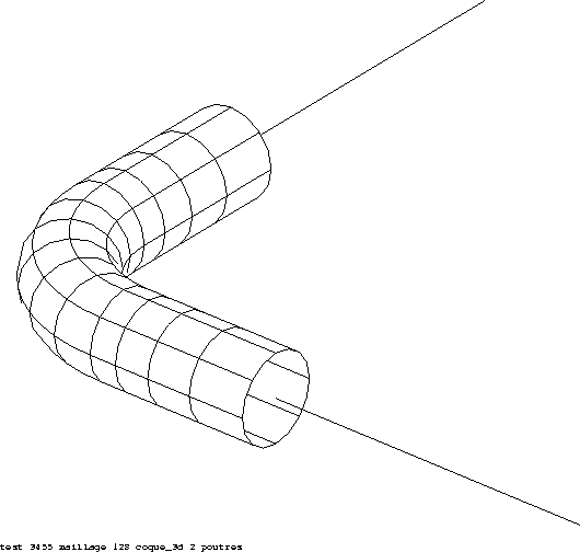
Figure 7.1-a: Connection between a mesh COQUE_3D and straight pipes [HI75-98/001]
Thanks to the kinematics introduced into the pipe element, the shell-pipe and 3D-pipe connections must allow the elbow to be meshed into shell elements or in 3D only, without straight parts, since the damping of ovalization (and warping) is taken into account in the pipe element.
The connection results in kinematic relationships between the degrees of freedom of the \(S\) nodes (which represents the connection section, modeled by shell edge or 3D elements), and the pipe node \(N\).
For the link to be effective, it must [R3.03.03] verify the following properties:
to be able to transmit beam forces to the shell or 3D mesh, and to be able to transmit all the degrees of freedom of the pipe element (or the dual forces of these),
do not create parasitic stresses in shell or 3D elements,
do not favor kinematic relationships or static conditions in relation to each other,
admit any behaviors and function dynamically.
The linear relationships will have the same form as in the shell-beam case, with additional equations specific to the degrees of freedom of the pipe.
We have already introduced to [§3.1] the space \(T\) of the fields associated with a torsor (defined by two vectors):
\(T=\left\{v\in V/\exists (T,\Omega )\text{tel que}v(M)=T+\Omega \wedge \text{GM}\right\}\)
where for the displacement fields of \(T\), \(T\) is the translation of the section (or of the point \(G\)), \(\Omega\) is the infinitesimal rotation and the fields
are the displacements maintaining the section \(S\) flat and not deformed (Here again we use the hypotheses of NAVIER - BERNOULLI).
The displacement of the pipe is then equal to:
\(\begin{array}{ccc}{u}^{t}={u}^{p}+{u}^{s}& {u}^{p}\in T& ,{u}^{s}\in {T}^{\perp }\end{array}\)
where:
\({T}^{\perp }=\left\{v\in V/\underset{S}{\int }v\text{.}w=0\forall w\in T\right\}\)
The approach consists in decomposing the shell displacement field \({u}^{c}\) or the three-dimensional displacement field \({u}^{\mathrm{3d}}\) into three fields:
\({u}^{c}={u}^{p}+{u}^{s}+{u}^{\epsilon }\)
a field of movement according to the kinematics of a \({u}^{p}\) beam (twister),
a local displacement field of the section according to pipe kinematics \({u}^{s}\) (Fourier series) defined in [§3.1],
an additional field \({u}^{\epsilon }\) orthogonal to the first two in the sense of dot product.
Note:
When the Fourier series decomposition of [§3.1] is infinite we have \({u}^{\epsilon }=0\) .
To translate the above equation into linear relationships, we show that it is necessary to calculate the following integrals, for the shell (or the 3D) and the pipe:
average displacement: \({\int }_{S}{u}^{c}\text{dS}\)
average rotation: \({\int }_{S}\text{GM}\wedge {u}^{c}\text{dS}\)
medium swelling: \({\int }_{S}\frac{\text{GM}}{\parallel \text{GM}\parallel }\text{.}{u}^{c}\text{dS}\)
Fourier modes: \({\int }_{S}{u}^{c}\text{cos}\mathrm{p\phi }\text{dS},{\int }_{S}{u}^{c}\text{sin}\mathrm{p\phi }\text{dS}\), \({\int }_{S}{u}^{c}\wedge \frac{\text{GM}}{\parallel \text{GM}\parallel }\text{cos}\mathrm{p\phi }\text{dS}\), \({\int }_{S}{u}^{c}\wedge \frac{\text{GM}}{\parallel \text{GM}\parallel }\text{sin}\mathrm{p\phi }\text{dS}\),,, \({\int }_{S}\frac{\text{GM}}{\parallel \text{GM}\parallel }\text{.}{u}^{c}\text{cos}\mathrm{p\phi }\text{dS}\), \({\int }_{S}\frac{\text{GM}}{\parallel \text{GM}\parallel }\text{.}{u}^{c}\text{sin}\mathrm{p\phi }\text{dS}\). For Fourier modes, we will choose the relationships that are easiest to use since some are redundant (see note from [§6.7]).
Note:
It is easy to switch from the analytical expressions of the 3D pipe connection to those of the shell - pipe connection. All you have to do is substitute \({u}^{\mathrm{3d}}\) to \({u}^{c}\) in all of the connection integrals proposed above. We will therefore only talk about this connection again in [§7.8] dealing with digital implementation.
7.2. Pipe kinematics.#
In the curvilinear base \((o,x,y,z)\) associated with the transverse section of [§2.1] we note the displacements \({u}_{1},{u}_{2}\text{et}{u}_{3}\) where:
\(\begin{array}{}{u}_{1}(r,x,\phi )={u}_{x}(x)-{\theta }_{y}(x)r\text{cos}\phi +{\theta }_{z}(x)r\text{sin}\phi +u(x,\phi )+\zeta {\beta }_{\phi }(x,\phi )\\ {u}_{2}(r,x,\phi )={u}_{y}(x)+{\theta }_{x}(x)r\text{cos}\phi -v(x,\phi )\text{cos}\phi -w(x,\phi )\text{sin}\phi +\zeta {\beta }_{\theta }(x,\phi )\text{cos}\phi \\ {u}_{3}(r,x,\phi )={u}_{z}(x)-{\theta }_{x}(x)r\text{sin}\phi +v(x,\phi )\text{sin}\phi -w(x,\phi )\text{cos}\phi -\zeta {\beta }_{\theta }(x,\phi )\text{sin}\phi \end{array}\).
Once discretized, this expression becomes:
\(\begin{array}{}{u}_{1}(r,x,\phi )={\sum }_{k=1}^{N}{H}_{k}(x)({x}_{k}\cdot x){u}_{x}^{k}+{H}_{k}(x)({y}_{k}\cdot x){u}_{y}^{k}-\stackrel{ˉ}{{H}_{k}}(x)({x}_{k}\cdot y){\theta }_{y}^{k}r\mathrm{cos}\phi -\stackrel{ˉ}{{H}_{k}}(x)({y}_{k}\cdot y){\theta }_{y}^{k}r\mathrm{cos}\phi +\stackrel{ˉ}{{H}_{k}}(x){\theta }_{z}^{k}r\mathrm{sin}\phi +u(x,\phi )+\zeta {\beta }_{\phi }(x,\phi )\\ {u}_{2}(r,x,\phi )={\sum }_{k=1}^{N}\stackrel{ˉ}{{H}_{k}}(x)({x}_{k}\cdot y){u}_{x}^{k}+{H}_{k}(x)({y}_{k}\cdot y){u}_{y}^{k}+\stackrel{ˉ}{{H}_{k}}(x)({x}_{k}\cdot x){\theta }_{x}^{k}r\mathrm{cos}\phi +\stackrel{ˉ}{{H}_{k}}(x)({y}_{k}\cdot x){\theta }_{y}^{k}r\mathrm{cos}\phi -v(x,\phi )\mathrm{cos}\phi -w(x,\phi )\mathrm{sin}\phi +\zeta {\beta }_{\theta }(x,\phi )\mathrm{cos}\phi \\ {u}_{3}(r,x,\phi )={\sum }_{k=1}^{N}{H}_{k}(x){u}_{z}^{k}-\stackrel{ˉ}{{H}_{k}}(x)({x}_{k}\cdot x){\theta }_{x}^{k}r\mathrm{sin}\phi -\stackrel{ˉ}{{H}_{k}}(x)({y}_{k}\cdot x){\theta }_{y}^{k}r\mathrm{sin}\phi +v(x,\phi )\mathrm{sin}\phi -w(x,\phi )\mathrm{cos}\phi -\zeta {\beta }_{\theta }(x,\phi )\mathrm{sin}\phi \end{array}\)
where \(u(x,\phi ),v(x,\phi ),w(x,\phi ),{\beta }_{\theta }(x,\phi )\text{et}{\beta }_{\theta }(x,\phi )\) are discretized as in [§3.1].
The displacement to a node \(k\) of abscissa \({x}_{k}\) end of pipe is then written:
\(\begin{array}{cc}{u}_{1}(r,{x}_{k},\phi )=& {u}_{x}^{k}-{\theta }_{y}^{k}r\mathrm{cos}(\phi )+{\theta }_{z}^{k}r\mathrm{sin}(\phi )+{\sum }_{m=2}^{M}({u}_{\mathrm{km}}^{i}\mathrm{cos}m\phi +{u}_{\mathrm{km}}^{0}\mathrm{sin}m\phi )+\zeta {\beta }_{\phi }({x}_{k},\phi )\\ {u}_{2}(r,{x}_{k},\phi )=& {u}_{y}^{k}+{\theta }_{x}^{k}r\mathrm{cos}(\phi )-\mathrm{cos}\phi {\sum }_{m=2}^{M}({v}_{\mathrm{km}}^{i}\mathrm{sin}m\phi +{v}_{\mathrm{km}}^{0}\mathrm{cos}m\phi )-\mathrm{sin}\phi {\sum }_{m=2}^{M}({w}_{\mathrm{km}}^{i}\mathrm{cos}m\phi +{w}_{\mathrm{km}}^{0}\mathrm{sin}m\phi )\\ & -{w}_{\mathrm{k1}}^{i}\mathrm{sin}2\phi +{w}_{\mathrm{k1}}^{0}\mathrm{cos}2\phi -{w}_{k}^{0}\mathrm{sin}\phi +\zeta {\beta }_{\theta }({x}_{k},\phi )\mathrm{cos}\phi \\ {u}_{3}(r,{x}_{k},\phi )=& {u}_{z}^{k}-{\theta }_{x}^{k}r\mathrm{sin}(\phi )+\mathrm{sin}\phi {\sum }_{m=2}^{M}({v}_{\mathrm{km}}^{i}\mathrm{sin}m\phi +{v}_{\mathrm{km}}^{0}\mathrm{cos}m\phi )-\mathrm{cos}\phi {\sum }_{m=2}^{M}({w}_{\mathrm{km}}^{i}\mathrm{cos}m\phi +{w}_{\mathrm{km}}^{0}\mathrm{sin}m\phi )\\ & -{w}_{\mathrm{k1}}^{i}\mathrm{cos}2\phi -{w}_{\mathrm{k1}}^{0}\mathrm{sin}2\phi -{w}_{k}^{0}\mathrm{cos}\phi -\zeta {\beta }_{\theta }({x}_{k},\phi )\mathrm{sin}\phi \end{array}\)
For the pipe, the angular momentum vector \(\text{GM}\wedge u(M)\) and the swelling \(\frac{\text{GM}}{\parallel \text{GM}\parallel }\text{.}u(M)\) have the following expressions, respectively:
\(\text{GM}\wedge u(M)=\{\begin{array}{c}-{u}_{z}(x)r\text{sin}\phi +{u}_{y}(x)r\text{cos}\phi +{r}^{2}{\theta }_{x}(x)-\text{rv}(x,\phi )\\ -{\text{ru}}_{1}(r,x,\phi )\text{cos}\phi \\ {\text{ru}}_{1}(r,x,\phi )\text{sin}\phi \end{array}\),
and:
\(\frac{\text{GM}}{\parallel \text{GM}\parallel }\text{.}u(M)=-{u}_{z}(x)\text{cos}\phi -{u}_{y}(x)\text{sin}\phi +w(x,\phi )\).
Note:
The first component of the field of movement uses \(u(x,\phi )\) in isolation. The same goes for the first component of the rotation vector vis-a-vis to \(v(x,\phi )\) *and of the swelling vis-a-vis \(w(x,\phi )\). This note will be used in [§5.6] to link Fourier modes to shell edge degrees of freedom.
7.3. Shell kinematics#
The Love-Kirchhoff or Naghdi-Mindlin shell kinematics is written in the thickness:
\({u}^{c}(M)={u}^{c}(Q)+({\theta }^{c}(Q)\wedge n)\text{.}{y}_{3}\)
\({u}^{c}(Q)\) is the displacement vector of the mean surface in \(Q\),
\({\theta }^{c}(Q)\) is the rotation vector in \(Q\) of the normal in the directions \({t}_{1}\) and \({t}_{2}\) of the tangential plane to \(Q\).
This displacement and rotation are calculated in the global coordinate system. By changing the coordinate system, it is possible to have their expressions in the curvilinear base \((o,x,y,z)\) of [§2.1] associated with the cross section of the junction between the shell and the pipe.
For each node, the program calculates the coefficients of the \(9+6(M\mathrm{-}1)\) linear relationships that connect:
the 6 degrees of freedom of the pipe’s \(P\) beam node,
the \(2+3\mathrm{\times }2(M\mathrm{-}1)\) Fourier degrees of freedom of the pipe,
the degree of freedom of swelling of the pipe,
with the degrees of freedom of all the nodes in the shell edge mesh list.
These linear relationships will be dualized, like all linear relationships derived for example from the LIAISON_DDL keyword in AFFE_CHAR_MECA. They are built as for the 3D-beam connection from the assembly of elementary terms.
7.4. Calculation of the average displacement on the S section#
The aim is to calculate the integral \({\int }_{S}{u}^{c}\text{dS}\), where \({u}^{c}\) is the shell displacement (with 6 ddl per node), \(S\) is the shell edge.
The average displacement on section \(S\) is written as:
\({\int }_{S}{u}^{c}(M)\text{dS}=h{\int }_{l}{u}^{c}(Q)\text{dl}+{\int }_{l}({\theta }^{c}(Q)\wedge n)({\int }_{-h/2}^{h/2}{y}_{3}{\text{dy}}_{3})\text{dl}\)
be \({\int }_{S}{u}^{c}(M)\text{dS}=h{\int }_{l}{u}^{c}(Q)\text{dl}\).
In addition, for the pipe part, we also have:
\({\int }_{S}{u}^{c}(M)\text{dS}={\int }_{S}[{u}^{p}(M)+{u}^{s}(M)]\text{dS}=\underset{S}{\int }(\begin{array}{c}{u}_{x}^{k}\\ {u}_{y}^{k}\\ {u}_{z}^{k}\end{array})\text{dS}=S(\begin{array}{c}{u}_{x}^{k}\\ {u}_{y}^{k}\\ {u}_{z}^{k}\end{array})\).
It is thus established that the average displacement of the pipe section at node \(k\) is equal to the beam displacement of node \(k\). It is thus possible to linearly link the degrees of freedom of the translation beam at node \(k\) with the average of the degrees of freedom of movement of the edge of the shell.
In this expression, the metric variation in the thickness of the shell is overlooked.
7.5. Calculation of the average rotation of the S section#
\(\begin{array}{}{\int }_{S}\text{GM}\wedge {u}^{c}(M)\text{dS}={\int }_{l}{\int }_{-h/2}^{h/2}(\text{GQ}+{y}_{3}n(Q))\wedge ({u}^{c}(Q)+{\theta }^{c}(Q)\wedge n(Q){y}_{3})\text{dl}{\text{dy}}_{3}\\ =h{\int }_{l}\text{GQ}\wedge {u}^{c}(Q)\text{dl}+{\int }_{l}\text{GQ}\wedge ({\theta }^{c}(Q)\wedge n(Q))\text{dl}{\int }_{-h/2}^{h/2}{y}_{3}{\text{dy}}_{3}\\ +{\int }_{l}n(Q)\wedge {u}^{c}(Q)({\int }_{-h/2}^{h/2}{y}_{3}{\text{dy}}_{3})\text{dl}+{\int }_{l}n(Q)\wedge ({\theta }^{c}(Q)\wedge n(Q)){\int }_{-\frac{h}{2}}^{\frac{h}{2}}{y}_{3}^{2}{\text{dy}}_{3}\text{.}\text{dl}\end{array}\)
be \({\int }_{S}\text{GM}\wedge {u}^{c}(M)\text{.}\text{dS}=h{\int }_{l}\text{GQ}\wedge {u}^{c}(Q)\text{dl}+\frac{{h}^{3}}{\text{12}}{\int }_{l}{\theta }^{c}(Q)\text{dl}\).
In addition, for the pipe part, we also have:
\({\int }_{S}\text{GM}\wedge {u}^{c}(M)\mathrm{.}\text{dS}={\int }_{S}\text{GM}\wedge \left[{u}^{p}(M)+{u}^{s}(M)\right]\mathrm{.}\text{dS}={\int }_{S}(\begin{array}{c}{r}^{2}\mathrm{.}{\theta }_{x}^{k}\\ {r}^{2}\mathrm{.}{\mathrm{cos}}^{2}\phi {\theta }_{y}^{k}\\ {r}^{2}\mathrm{.}{\mathrm{sin}}^{2}\phi {\theta }_{z}^{k}\end{array})=I(\begin{array}{c}{\theta }_{x}^{k}\\ {\theta }_{y}^{k}\\ {\theta }_{z}^{k}\end{array})\)
where*I* is the inertia tensor of the beam. It is thus established that the average rotation of the pipe section at node \(k\) is equal to the rotation of the beam at node \(k\). It is thus possible to linearly link the degrees of freedom of the rotation beam at node \(k\) with the degrees of freedom of rotation of the edge of the shell.
In this expression, the metric variation in the thickness of the shell is overlooked.
7.6. Calculation of the average swelling of section S#
The aim is to calculate the integral \({\int }_{S}{u}^{c}\text{.}n\text{dS}={\int }_{S}{u}^{c}\text{.}\frac{\text{GM}}{\parallel \text{GM}\parallel }\text{dS}\), where \(n=\frac{\text{GM}}{\parallel \text{GM}\parallel }=\frac{\text{GQ}}{\parallel \text{GQ}\parallel }\) is the normal to the mean shell area.
The average displacement on section \(S\) is written as:
\({\mathrm{\int }}_{S}{u}^{c}(M)\text{.}n\text{dS}\mathrm{=}h{\mathrm{\int }}_{l}{u}^{c}(Q)\text{.}n\text{dl}+{\mathrm{\int }}_{l}({\theta }^{c}(Q)\mathrm{\wedge }n)\text{.}n({\mathrm{\int }}_{\mathrm{-}h\mathrm{/}2}^{h\mathrm{/}2}{y}_{3}{\text{dy}}_{3})\text{dl}\mathrm{=}h{\mathrm{\int }}_{l}{u}^{c}(Q)\text{.}n\text{dl}\).
In addition, for the pipe part, we also have:
\({\mathrm{\int }}_{S}\frac{\text{GM}}{\mathrm{\parallel }\text{GM}\mathrm{\parallel }}\text{.}{u}^{c}(M)\text{dS}\mathrm{=}{\mathrm{\int }}_{S}\frac{\text{GM}}{\mathrm{\parallel }\text{GM}\mathrm{\parallel }}\text{.}\mathrm{[}{u}^{p}(M)+{u}^{s}(M)\mathrm{]}\text{dS}\mathrm{=}\underset{S}{\mathrm{\int }}{w}_{k}^{o}\text{dS}\)
It is thus established that the average swelling of the pipe section at node \(k\) is equal to the degree of freedom of swelling of the pipe at node \(k\). It is thus possible to linearly link the degree of freedom of pipe swelling at node \(k\) with the degrees of freedom of movement of the edge of the shell.
In this expression, the metric variation in the thickness of the shell is overlooked.
7.7. Calculation of Fourier coefficients on section S#
The aim is to calculate the six integrals \({\int }_{S}{u}^{c}\text{cos}\mathrm{p\phi }\text{dS}\), \({\int }_{S}{u}^{c}\text{sin}\mathrm{p\phi }\text{dS}\), \({\int }_{S}{u}^{c}\wedge \frac{\text{GM}}{\parallel \text{GM}\parallel }\text{cos}\mathrm{p\phi }\text{dS}\),, \({\int }_{S}{u}^{c}\wedge \frac{\text{GM}}{\parallel \text{GM}\parallel }\text{sin}\mathrm{p\phi }\text{dS}\),, \({\int }_{S}\frac{\text{GM}}{\parallel \text{GM}\parallel }\text{.}{u}^{c}\text{cos}\mathrm{p\phi }\text{dS}\) and \({\int }_{S}\frac{\text{GM}}{\parallel \text{GM}\parallel }\text{.}{u}^{c}\text{sin}\mathrm{p\phi }\text{dS}\), where \({u}^{c}\) is the shell displacement (with 6 ddl per node), \(S\) is the shell edge.
We have the following relationship for trips on section \(S\):
\({\int }_{S}{u}^{c}(M)\text{cos}\mathrm{p\phi }\text{dS}=h{\int }_{l}{u}^{c}(Q)\text{cos}\mathrm{p\phi }\text{dl}+{\int }_{l}({\theta }^{c}(Q)\wedge n)({\int }_{-h/2}^{h/2}{y}_{3}{\text{dy}}_{3})\text{cos}\mathrm{p\phi }\text{dl}\)
either \({\int }_{S}{u}^{c}(M)\text{cos}\mathrm{p\phi }\text{dS}=h{\int }_{l}{u}^{c}(Q)\text{cos}\mathrm{p\phi }\text{dl}\) and \({\int }_{S}{u}^{c}(M)\text{sin}\mathrm{p\phi }\text{dS}=h{\int }_{l}{u}^{c}(Q)\text{sin}\mathrm{p\phi }\text{dl}\).
In addition, for the pipe part, we also have:
\({\int }_{S}{u}^{c}(M)\text{cos}\mathrm{p\phi }\text{dS}=\underset{S}{\int }(\begin{array}{c}{u}_{1}(r,{x}_{k},\phi )\\ {u}_{2}(r,{x}_{k},\phi )\\ {u}_{3}(r,{x}_{k},\phi )\end{array})\text{cos}\mathrm{p\phi }\text{dS}\).
The first component of this relationship then allows us to linearly relate Fourier coefficient \({u}_{\text{kp}}^{i}\) to the components of shell edge displacements in the following way:
\(h{\mathrm{\int }}_{l}{u}_{1}^{c}(Q)\text{cos}\mathit{p\phi }\text{dl}\mathrm{=}{\mathrm{\int }}_{S}{u}_{1}(r,{x}_{k},\phi )\text{cos}\mathit{p\phi }\text{dS}\mathrm{=}\mathrm{\{}\begin{array}{cc}\mathrm{-}\underset{S}{\mathrm{\int }}{\mathit{r\theta }}_{y}^{k}{\text{cos}}^{2}\phi \text{dS}& \text{si}p\mathrm{=}1\\ \underset{S}{\mathrm{\int }}{u}_{\text{kp}}^{i}{\text{cos}}^{2}\mathit{p\phi }\text{dS}& \text{si}p\mathrm{\ne }1\end{array}\)
Likewise \({\int }_{S}{u}^{c}(M)\text{sin}\mathrm{p\phi }\text{dS}=\underset{S}{\int }(\begin{array}{c}{u}_{1}(r,{x}_{k},\phi )\\ {u}_{2}(r,{x}_{k},\phi )\\ {u}_{3}(r,{x}_{k},\phi )\end{array})\text{sin}\mathrm{p\phi }\text{dS}\) from which we deduce that:
\(h{\int }_{l}{u}_{1}^{c}(Q)\text{sin}\mathrm{p\phi }\text{dl}={\int }_{S}{u}_{1}(r,{x}_{k},\phi )\text{sin}\mathrm{p\phi }\text{dS}=\{\begin{array}{cc}\underset{S}{\int }{\mathrm{r\theta }}_{z}^{k}{\text{sin}}^{2}\phi \text{dS}& \text{si}p=1\\ \underset{S}{\int }{u}_{\text{kp}}^{o}{\text{sin}}^{2}\mathrm{p\phi }\text{dS}& \text{si}p\ne 1\end{array}\begin{array}{c}\\ \end{array}\)
We have the following relationship for the rotations on section \(S\):
\({\int }_{S}{u}^{c}(M)\wedge \text{.}\frac{\text{GM}}{\parallel \text{GM}\parallel }\text{cos}\mathrm{p\phi }\text{dS}=h{\int }_{l}{u}^{c}(Q)\wedge \frac{\text{GQ}}{\parallel \text{GQ}\parallel }\text{cos}\mathrm{p\phi }\text{dl}+{\int }_{l}({\theta }^{c}(Q)\wedge n)\wedge n(\underset{-h/2}{\overset{+h/2}{\int }}{y}_{3}{\text{dy}}_{3})\text{cos}\mathrm{p\phi }\text{dl}\).
The first component of this relationship then allows us to linearly relate Fourier coefficient \({v}_{\text{kp}}^{o}\) to the components of the displacements and rotations of the shell edge in the following way:
\(h{\int }_{l}[{u}^{c}(Q)\wedge \frac{\text{GQ}}{\parallel \text{GQ}\parallel }{]}_{1}\text{cos}\mathrm{p\phi }\text{dl}=\{\begin{array}{cc}-\underset{S}{\int }[{\text{ru}}_{y}^{k}{\text{cos}}^{2}\phi +{\text{rw}}_{\mathrm{k1}}^{o}{\text{cos}}^{2}\phi ]\text{dS}& \text{si}p=1\\ \underset{S}{\int }{\text{rv}}_{\text{kp}}^{o}{\text{cos}}^{2}(\mathrm{p\phi })\text{dS}& \text{si}p\ne 1\end{array}\)
In the same way we have:
\(h{\int }_{l}[{u}^{c}(Q)\wedge \frac{\text{GQ}}{\parallel \text{GQ}\parallel }{]}_{1}\text{sin}\mathrm{p\phi }\text{dl}=\{\begin{array}{cc}\underset{S}{\int }[{\text{ru}}_{z}^{k}{\text{sin}}^{2}\phi +{\text{rw}}_{\mathrm{k1}}^{i}{\text{sin}}^{2}\phi ]\text{dS}& \text{si}p=1\\ \underset{S}{\int }{\text{rv}}_{\text{kp}}^{i}{\text{sin}}^{2}(\mathrm{p\phi })\text{dS}& \text{si}p\ne 1\end{array}\)
We have the following relationship for swelling on section \(S\):
\({\int }_{S}\frac{\text{GM}}{\parallel \text{GM}\parallel }\text{.}{u}^{c}(M)\text{.}\text{cos}\mathrm{p\phi }\text{dS}=h{\int }_{l}\frac{\text{GQ}}{\parallel \text{GQ}\parallel }\text{.}{u}^{c}(Q)\text{cos}\mathrm{p\phi }\text{dl}\).
This relationship allows us to linearly relate Fourier coefficient \({w}_{\text{kp}}^{i}\) to the components of shell edge displacements in the following way:
\(h{\mathrm{\int }}_{l}\frac{\text{GQ}}{\mathrm{\parallel }\text{GQ}\mathrm{\parallel }}\mathrm{.}{u}^{c}(Q)\text{cos}\mathit{p\phi }\text{dl}\mathrm{=}\mathrm{\{}\begin{array}{cc}\underset{S}{\mathrm{\int }}\mathrm{[}\mathrm{-}{u}_{z}^{k}{\text{cos}}^{2}\phi +{w}_{\mathit{k1}}^{i}{\text{cos}}^{2}\phi \mathrm{]}\text{dS}& \text{si}p\mathrm{=}1\\ \underset{S}{\mathrm{\int }}{w}_{\text{kp}}^{i}{\text{cos}}^{2}(\mathit{p\phi })\text{dS}& \text{si}p\mathrm{\ne }1\end{array}\).
Likewise, we have:
\(h{\int }_{l}\frac{\text{GQ}}{\parallel \text{GQ}\parallel }\mathrm{.}{u}^{c}(Q)\text{sin}\mathrm{p\phi }\text{dl}=\{\begin{array}{cc}\underset{S}{\int }-{u}_{y}^{k}{\text{sin}}^{2}\phi +{w}_{\mathrm{k1}}^{o}{\text{sin}}^{2}\phi \text{dS}& \text{si}p=1\\ \underset{S}{\int }{w}_{\text{kp}}^{o}{\text{sin}}^{2}(\mathrm{p\phi })\text{dS}& \text{si}p\ne 1\end{array}\)
For all these relationships, we use the fact that \(\underset{S}{\int }\text{cos}\mathrm{p\phi }\text{cos}\mathrm{q\phi }\text{dS}=0\text{si}p\ne q\text{.}\)
In this expression, the metric variation in the thickness of the shell is overlooked.
Note:
It should be noted that some of the relationships established in this paragraph for p=1 are redundant with those established in paragraphs [§7.4] and [§7.5]. Of the six relationships established from the calculation of the integral forms \({\int }_{S}{u}^{\mathrm{c.}}\mathrm{cos}\phi \mathrm{dS}\) , \({\int }_{S}{u}^{\mathrm{c.}}\mathrm{sin}\phi \mathrm{dS}\) , , \({\int }_{S}{u}^{c}\wedge \frac{\mathrm{GM}}{∥\mathrm{GM}∥}\mathrm{.}\mathrm{cos}\phi \mathrm{dS}\) , \({\int }_{S}{u}^{c}\wedge \frac{\mathrm{GM}}{∥\mathrm{GM}∥}\mathrm{.}\mathrm{sin}\phi \mathrm{dS}\) , \({\int }_{S}{u}^{c}\wedge \frac{\mathrm{GM}}{∥\mathrm{GM}∥}\mathrm{.}{u}^{c}\mathrm{cos}\phi \mathrm{dS}\) and \({\int }_{S}{u}^{c}\wedge \frac{\mathrm{GM}}{∥\mathrm{GM}∥}\mathrm{.}{u}^{c}\mathrm{sin}\phi \mathrm{dS}\), only two of the last four are linearly independent of the others. So the first two have already been established in [§7.4] and combinations of the last four restore those of [§7.5].
7.8. Implementation of the method#
The coefficients of linear relationships are calculated in three stages:
calculation of elementary quantities on the elements in the list of shell edge cells (mesh type SEG2):
area = \({\int }_{\text{elt}}1;{\int }_{\text{elt}}x;{\int }_{\text{elt}}y;{\int }_{\text{elt}}z\).
summation of these quantities on (\(S\)) hence the calculation of:
\(A=\mid S\mid\)
position of \(G\).
knowing \(G\), elementary calculation on the elements in the list of shell edge cells of:
\({\int }_{\text{elt}}\text{Ni};{\int }_{\text{elt}}\text{xNi};{\int }_{\text{elt}}\text{yNi};{\int }_{\text{elt}}\text{zNi}\text{où :}\begin{array}{c}\text{GM}=\left\{x,y,z\right\}\\ \text{Ni}=\text{fonctions de forme de l'élément}\end{array}\)
It should be noted that in the case of the shell-pipe connection, the integrals on the edge elements are to be multiplied by the thickness of the shell: \(\underset{\text{elt}}{\int }{N}_{i}=h\underset{l}{\int }{N}_{i}\) where \(l\) represents the average fiber of the shell edge element. In addition, we add the additional term: \(\frac{{h}^{3}}{\text{12}}\underset{l}{\int }{N}_{i}\).
« assembly » of the terms calculated above to obtain, at each of the nodes of the connection section, the coefficients of the terms of the linear relationships,
link between Fourier modes and shell movements as shown at the beginning of [§7].
More specifically:
for the shell-pipe connection, elementary calculations are carried out on all the edge elements of the connection section \(S\) of the type:
\({u}_{\text{cm}}=\frac{1}{\pi }\underset{0}{\overset{\mathrm{2\pi }}{\int }}{u}^{c}\text{cos}(m\varphi )d\varphi =\frac{1}{\pi }\underset{0}{\overset{\mathrm{2\pi }}{\int }}(\begin{array}{c}{u}_{{x}^{c}}\\ {u}_{{\varphi }^{c}}\\ {u}_{{r}^{c}}\end{array})\text{cos}(m\varphi )d\varphi =\frac{1}{\pi }\sum _{n=1}^{\text{Nb}\varphi \text{éléments}\in S}\underset{{\varphi }_{1}^{n}}{\overset{{\varphi }_{2}^{n}}{\int }}\text{cos}(m\varphi )P(\begin{array}{c}{u}_{{x}^{c}}\\ {u}_{{y}^{c}}\\ {u}_{{z}^{c}}\end{array})d\varphi\)
and
\({u}_{\text{sm}}=\frac{1}{\pi }\underset{0}{\overset{\mathrm{2\pi }}{\int }}{u}^{c}\text{sin}(m\varphi )d\varphi =\frac{1}{\pi }\underset{0}{\overset{\mathrm{2\pi }}{\int }}(\begin{array}{c}{u}_{{x}^{c}}\\ {u}_{{\varphi }^{c}}\\ {u}_{{r}^{c}}\end{array})\text{sin}(m\varphi )d\varphi =\frac{1}{\pi }\sum _{n=1}^{\text{Nb}\varphi \text{éléments}\in S}\underset{{\varphi }_{1}^{n}}{\overset{{\varphi }_{2}^{n}}{\int }}\text{sin}(m\varphi )P(\begin{array}{c}{u}_{{x}^{c}}\\ {u}_{{y}^{c}}\\ {u}_{{z}^{c}}\end{array})d\varphi\)
if \(m>1\) where \(P\) is the matrix for moving from the local coordinate system of the element to the global coordinate system and \({\varphi }_{1}\) is the orthoradial position of the element. By expressing the displacement as a function of the nodal degrees of freedom:
\({u}_{\text{cm}}=(\begin{array}{c}{u}_{m}^{i}\\ {v}_{m}^{o}\\ {w}_{m}^{i}\end{array})=\frac{1}{\pi }\sum _{n=1}^{\text{Nb}\varphi \text{éléments}\in S}\underset{{\varphi }_{1}^{n}}{\overset{{\varphi }_{2}^{n}}{\int }}\text{cos}(m\varphi )P\sum _{n=1}^{{\text{Nb}}_{\text{noeuds}}}{N}_{n}(\varphi )(\begin{array}{c}{U}_{{x}^{n}}\\ {U}_{{y}^{n}}\\ {U}_{{z}^{n}}\end{array})d\varphi\)
and
\({u}_{\text{sm}}=(\begin{array}{c}{u}_{m}^{o}\\ {v}_{m}^{i}\\ {w}_{m}^{o}\end{array})=\frac{1}{\pi }\sum _{n=1}^{\text{Nb}\varphi \text{éléments}\in S}\underset{{\varphi }_{1}^{n}}{\overset{{\varphi }_{2}^{n}}{\int }}\text{sin}(m\varphi )P\sum _{n=1}^{{\text{Nb}}_{\text{noeuds}}}{N}_{n}(\varphi )(\begin{array}{c}{U}_{{x}^{n}}\\ {U}_{{y}^{n}}\\ {U}_{{z}^{n}}\end{array})d\varphi\)
where \(N\) are the shape functions of the element, for each calculation we get two times 9 coefficients at the nodes of the current element of \(S\):
\(\begin{array}{}{u}_{\text{cm}}=(\begin{array}{c}{u}_{m}^{i}\\ {v}_{m}^{o}\\ {w}_{m}^{i}\end{array})=\left\{\sum _{\text{éléments}\in S}^{}\sum _{n=1}^{{\text{Nb}}_{\text{noeuds}}}(\begin{array}{ccc}{a}_{\text{11}}& {a}_{\text{12}}& {a}_{\text{13}}\\ {a}_{\text{21}}& {a}_{\text{22}}& {a}_{\text{23}}\\ {a}_{\text{31}}& {a}_{\text{32}}& {a}_{\text{33}}\end{array})\right\}(\begin{array}{c}{U}_{{x}^{n}}\\ {U}_{{y}^{n}}\\ {U}_{{z}^{n}}\end{array})\text{.}\\ {a}_{\text{ij}}^{n}=\frac{1}{\pi }\underset{{\varphi }_{1}}{\overset{{\varphi }_{2}}{\int }}\text{cos}(m\varphi ){P}_{\text{ij}}(\varphi ){N}_{n}(\varphi )d\varphi =\frac{1}{\mathrm{\pi R}}\underset{0}{\overset{l}{\int }}\text{cos}(\text{mx}){P}_{\text{ij}}(x){N}_{n}(x)\text{dx}\end{array}\)
and an equivalent expression for \({u}_{\mathrm{sm}}\) where \(I\) is the length of the shell edge element.
for the 3D - pipe connection, elementary calculations are carried out on all the edge elements of the connection section \(S\) of the type:
\(\begin{array}{c}{u}_{\text{cm}}\mathrm{=}\frac{2}{S}\underset{S}{\overset{}{\mathrm{\int }}}{u}^{\text{3d}}\text{cos}(m\varphi )\text{dS}\mathrm{=}\frac{2}{S}\underset{S}{\overset{}{\mathrm{\int }}}(\begin{array}{c}{u}_{{x}^{\text{3d}}}\\ {u}_{{\varphi }^{\text{3d}}}\\ {u}_{{r}^{\text{3d}}}\end{array})\text{cos}(m\varphi )r\mathrm{.}d\varphi \mathrm{.}\mathit{d\zeta }\\ \mathrm{=}\frac{2}{S}\mathrm{\sum }_{n\mathrm{=}1}^{\text{Nb}\varphi \text{éléments}\mathrm{\in }S}\underset{{\varphi }_{1}^{n}}{\overset{{\varphi }_{2}^{n}}{\mathrm{\int }}}\underset{{h}_{1}^{n}}{\overset{{h}_{2}^{n}}{\mathrm{\int }}}\text{cos}(m\varphi )P\mathrm{\sum }_{n\mathrm{=}1}^{{\text{Nb}}_{\text{noeuds}}}{N}_{n}(\varphi ,\zeta ){(\begin{array}{c}{U}_{x}^{\mathrm{3d}}\\ {U}_{y}^{\mathrm{3d}}\\ {U}_{z}^{\mathrm{3d}}\end{array})}^{n}r\mathrm{.}d\varphi \mathrm{.}\mathit{d\zeta }\end{array}\)
and
\(\begin{array}{c}{u}_{\text{sm}}\mathrm{=}\frac{2}{S}\underset{S}{\overset{}{\mathrm{\int }}}{u}^{\text{3d}}c\text{sin}(m\varphi )\text{dS}\mathrm{=}\frac{2}{S}\underset{S}{\overset{}{\mathrm{\int }}}(\begin{array}{c}{u}_{{x}^{\text{3d}}}\\ {u}_{{\varphi }^{\text{3d}}}\\ {u}_{{r}^{\text{3d}}}\end{array})\text{sin}(m\varphi )r\mathrm{.}d\varphi \mathrm{.}\mathit{d\zeta }\\ \mathrm{=}\frac{2}{S}\mathrm{\sum }_{n\mathrm{=}1}^{\text{Nb}\varphi \text{éléments}\mathrm{\in }S}\underset{{\varphi }_{1}^{n}}{\overset{{\varphi }_{2}^{n}}{\mathrm{\int }}}\underset{{h}_{1}^{n}}{\overset{{h}_{2}^{n}}{\mathrm{\int }}}\text{sin}(m\varphi )P\mathrm{\sum }_{n\mathrm{=}1}^{{\text{Nb}}_{\text{noeuds}}}{N}_{n}(\varphi ,\zeta ){(\begin{array}{c}{U}_{x}^{\mathrm{3d}}\\ {U}_{y}^{\mathrm{3d}}\\ {U}_{z}^{\mathrm{3d}}\end{array})}^{n}\mathit{r.}d\varphi \mathrm{.}\mathit{d\zeta }\end{array}\)
if \(m>1\) where \(P\) is the matrix for moving from the local coordinate system of the element to the global coordinate system, \({\varphi }_{1}\) the orthoradial position of the element, \({h}_{1}\) its radial position and the \(N\) are the shape functions of the element.