1. Introduction

There are several ways to define what a plate or shell is. We are going to adopt the following definition: « a plate (or a shell) is a mechanical structure, which « seen from a distance » is a surface ».

In practice, this will mean that one of its dimensions (its thickness) is negligible compared to the other two. More fundamentally, from a mathematical point of view, only curvature is a parameter that makes it possible to apply or not a shell theory; its thickness is not a founding hypothesis of the theory.

The distinction between plate ( »plate ») and shell ( »shell ») is based on the idea that the plate is an initially flat structure while the shell is a fundamentally curved structure. To represent a curved component (cylinder for example), plate elements therefore proceed by « facetting » the surface, which introduces both a geometric error (approximation of the curvature) but also a mechanical error since, for isotropic behaviors, this implies that the plates do not have a coupling between membrane and flexural deformations.

In general, a thin structure has a remarkable property: its mechanical strength (its balance) depends essentially on its geometry. There is a very strong difference in stiffness between stress in its average surface (membrane) and normal to its average surface (essentially bending). A thin structure is in fact much more rigid in membrane than in flexure (it is much easier to deform a sheet by folding it than by extending it).

In practice, this property will induce a lot of modeling problems, a series of numerical « locks », i.e. a poor representation of the various mechanical situations that cannot always be overcome by refining the mesh. The problem is fundamental and we are going to review the different situations that present these lockdowns and the ways to remove them.

1.1. Limitation of classical isoparametric elements

Classic 3D isoparametric elements present a series of numerical interlocks, due either to the poor representation of the various modes of deformation and stresses representative of thin structures, or to properties of the material or behavior (such as incompressibility or plasticity).

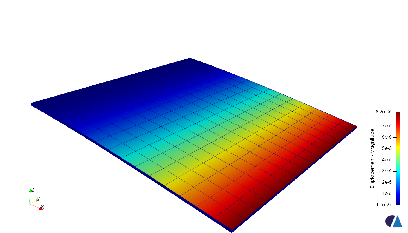
To illustrate the locking situations coming from the thin structure hypothesis, we will consider the calculation of a simple square plate in bending, represented by a single layer of 8-node cube-type elements (with therefore a tri-linear approximation of the displacements).

	Structure PropertiesGrade: \(1m\) Thickness: \(\mathrm{0,1}m\) Young’s Modulus: Young’s Modulus: \(210\mathit{GPa}\) Poisson’s Ratio: \(\mathrm{0,3}\)
Figure 1.1-1: Example of thin structure calculation in 3D

The maximum vertical displacement that should be obtained, based on the theory of thin plates (result obtained with elements DKT for example) is 1.9 mm.

On the 3D mesh:

Number of elements	Movement
Plate theory	\(\mathrm{1,9}\mathit{mm}\)
3D — 25	\(\mathrm{9,7}\times {10}^{-4}\mathit{mm}\)
3D — 2250	\(\mathrm{8,2}\times {10}^{-3}\mathit{mm}\)
3D — 75000	\(\mathrm{6,3}\times {10}^{-2}\mathit{mm}\)

We can see that we have a very small (and false) displacement and that we are only converging very slowly towards the right displacement. This is called a « lockdown. »

1.1.1. Shear locking

The previous plate is considered to be in pure bending. In this configuration, the solution of a beam model (it’s the same thing in plates, we just consider independence from the coordinate \(y\) to simplify the explanation) is as follows:

(1.1)\[\begin{split} \ {\ begin {array} {c} {\ epsilon} _ {\ mathit {xx}}} ^ {\ mathit {beam}} =\ frac {M} {\ mathit {EI}}} z\\ {\ epsilon}} z\\ {\ epsilon}} _ _ {\ mathit {zz}} _ {\ mathit {zz}}} ^ {\ mathit {zz}}} ^ {\ mathit {beam}}} =-\ frac {M\nu}} z\\ {\ epsilon}} z\\ {\ epsilon}} _ {\ mathit {zz}} _ {\ mathit {zz}}} ^ {\ mathit {zz}}} ^ {\ mathit {beam}}} =-\ frac {M\nu}} z=-\nu {\ epsilon} _ {\ mathit {xx}}} ^ {\ mathit {beam}}\\ {\ gamma} _ {\ mathit {xz}}} ^ {\ mathit {xz}}} ^ {\ mathit {beam}}} ^ {\ mathit {beam}} =0\ end {array}}\end{split}\]

Assuming \(\nu =0\) at first:

(1.2)\[\begin{split} \ {\ begin {array} {c} {\ epsilon} _ {\ mathit {xx}} _ {\ mathit {xx}}} ^ {\ mathit {beam}} =\ frac {M} {\ mathit {EI}}} z\\ {\ epsilon}} z\\ {\ epsilon}} _ {\ epsilon} _ {\ epsilon} _ {\ epsilon} _ {\ epsilon} _ {\ epsilon} _ {\ epsilon} _ {\ epsilon} _ {\ epsilon} _ {\ epsilon} _ {\ epsilon} _ {\ epsilon} _ {\ epsilon} _ {\ epsilon} _ {\ epsilon} _ {\ epsilon} _ {\ epsilon} ^ {\ mathit {beam}}} =0\ end {array}\end{split}\]

Now let’s look at the linear approximation in 3D. When flexing and considering independence with respect to \(y\) and complete 3D linear functions in the \((x,z)\) plane, the displacements are written as:

(1.3)\[\begin{split} \ left\ {\ begin {array} {c} {u} {u} {u} ^ {3D}\\ {W}} ^ {3D}\ end {array}\ right\} =\ left\ {\ begin {array} {c} {C} {C} {C} {C} {C}} =\ {7}\ mathit {xz} {C} {C} {7}\ mathit {xz} {C} {C} _ {2} + {C} _ {4} x+ {C} _ {6} z+ {C} _ {8}\ mathit {xz}\ end {array}\ end {array}\ right\}\end{split}\]

The three deformations are thus calculated:

\[\]

: label: eq-4

{begin {array} {c} {epsilon} _ {mathit {xx}} _ {xx}} ^ {3D} = {C} _ {3} + {C} _ {7} z\ {epsilon}} _ {epsilon} _ {epsilon} _ {epsilon} _ {epsilon} _ {epsilon} _ {gamma} _ {gamma} _ {zz}}} ^ {3D}} = {C} _ {6} + {C} _ {8} x{epsilon}} _ {epsilon} _ {gamma} _ {gamma} _ {gamma}} _ {mathit}}} ^ {3D}} = {C} _ {6}} + {C} _ {8} x{xz}} ^ {3D} = {C} _ {4} + {C} _ {5} + {C} _ {7} x+ {C} _ {C} _ {8} zend {array}

In fact, the eight coefficients \({C}_{i}\) correspond to particular deformation modes as summarized in the following table.

	Rigid \(x\)	Rigid \(z\)	Membrane \(x\)	Membrane \(z\)	Shear \(x\)	Shear \(z\)	Flexion \(x\)	Flexion \(z\)
\({u}^{3D}\)	\(C\mathrm{₁}\)	0	\(C\mathrm{₃}x\)		0	0	\(C\mathrm{₅}z\)	\(C\mathrm{₇}\mathit{xz}\)	0
\({w}^{3D}\)	0	\(C\mathrm{₂}\)	0	0	\(C\mathrm{₆}z\)		\(C\mathrm{₄}x\)	0	0	\(C\mathrm{₈}\mathit{xz}\)
\({\epsilon }_{\mathit{xx}}^{3D}\)	0	0	0	\(C\mathrm{₃}\)		0	0	\(C\mathrm{₇}z\)	0
\({\epsilon }_{\mathit{zz}}^{3D}\)	0	0	0	0	0	\(C\mathrm{₆}\)	0	0	\(C\mathrm{₈}x\)
\({\gamma }_{\mathit{xz}}^{3D}\)	0	0	0	0	0	0	\(C\mathrm{₄}\)	\(C\mathrm{₅}\)	\(C\mathrm{₇}x\)	\(C\mathrm{₈}z\)

The first two columns correspond to zero deformations, so they are rigid body movements (following \(x\) or following \(z\)). The next two have constant \({\epsilon }_{\mathit{xx}}^{3D}\) and \({\epsilon }_{\mathit{zz}}^{3D}\) deformations, they are pure membrane deformations, the next two corresponding to a non-zero \({\gamma }_{\mathit{xz}}^{3D}\) deformation (pure shear). Finally, the last two correspond to a bending strain (with shear).

If we consider the case of pure flexure (without membrane or shear components) the three-dimensional deformations are:

\[\]

: label: eq-5

{begin {array} {c} {epsilon} _ {mathit {xx}}} ^ {3D} = {C} _ {7} z\ {epsilon} _ {mathit {zz}}} ^ {zz}}} ^ {zz}} ^ {epsilon}} _ {7}} ^ {epsilon}} _ {7}} ^ {7} xend {array}} ^ {3D} = {C} _ {7}}} ^ {7} xend {array}}

Compared to the beam solution (see ()), we can see that the shear component \({\gamma }_{\mathit{xz}}^{3D}\) is not zero in 3D, this is what is called shear locking.

1.1.2. Pinch lock

Strictly speaking, this is not a lock because most of the plate models used in calculation (Kirchhoff, Mindlin) assume the inextensibility of the transverse fiber (the thickness) \({\epsilon }_{\mathit{zz}}=0\). But in some plate/shell models (Cosserat model for example), this hypothesis is not retained.

The conjunction of this hypothesis with that usually applied of plane stresses leads to a theoretical inconsistency in plate formulations. In fact, Hooke’s elasticity does not allow, in theory, to have \({\sigma }_{\mathit{zz}}=0\) and \({\epsilon }_{\mathit{zz}}=0\) simultaneously. However, this apparent contradiction disappears indirectly by the application of the variational formulation, and, from the mechanical point of view, by the fact that the hypothesis of plane constraints is « excessive »: one can neglect constraints \({\sigma }_{\mathrm{.}z}\) in relation to the others. Taking them to zero is a practical convenience.

For the most general plaque theories, remember that we have:

(1.4)\[\begin{split} \ {\ begin {array} {c} {\ epsilon} _ {\ mathit {xx}}} ^ {\ mathit {beam}} =\ frac {M} {\ mathit {EI}}} z\\ {\ epsilon}} z\\ {\ epsilon}} _ _ {\ mathit {zz}} _ {\ mathit {zz}}} ^ {\ mathit {zz}}} ^ {\ mathit {beam}}} =-\ frac {M\nu}} z\\ {\ epsilon}} z\\ {\ epsilon}} _ {\ mathit {zz}} _ {\ mathit {zz}}} ^ {\ mathit {zz}}} ^ {\ mathit {beam}}} =-\ frac {M\nu}} z=-\nu {\ epsilon} _ {\ mathit {xx}}} ^ {\ mathit {beam}}\\ {\ gamma} _ {\ mathit {xz}}} ^ {\ mathit {xz}}} ^ {\ mathit {beam}}} ^ {\ mathit {beam}} =0\ end {array}}\end{split}\]

And we can see in equation () that the expression for \({\epsilon }_{\mathit{zz}}^{\mathit{poutre}}\) is not found in 3D and is equal to:

(1.5)\[ {\ epsilon} _ {\ mathit {zz}}} ^ {3D} = {C} _ {6} + {C} _ {8} x\]

The deformation only depends on \(x\) and it is constant in thickness (hypothesis of the inextensibility of the normal fiber). One of the contributions of element COQUE_SOLIDE will be to correct this point and therefore to be a richer plate formulation than the others available in code_aster such as DKT, COQUE_3D, etc.

1.1.3. Membrane locking

Now consider a curved bending beam of length \(2l\) and radius \(R\), we have:

(1.6)\[\begin{split} \ {\ begin {array} {c} {\ epsilon} {\ epsilon} ^ {\ mathit {beam}} =\ frac {\ mathit {ds}}} +\ frac {w} {R}\\ epsilon}} ^ {\\ chi} ^ {\ mathit {beam}} =\ frac {\ mathit {of}}} {\ mathit {ds} {R}}\ frac {1} {R} -\ frac {{d} ^ {2} w} {{\ mathit {ds}} ^ {2}}}\ end {array}}\end{split}\]

Given the differentiability conditions, we must have the following approximations:

(1.7)\[ \ {\ begin {array} {c} u= {a} _ {a} _ {0} + {0} + {0} + {a} _ {0} + {b} _ {1}\ xi + {b} _ {b} _ {2} {\ xi} _ {2} {\ xi} ^ {3}\ end {array} _ {1}\ end {array} _ {1}\ xi} _ {1}\ xi} _ {1}\ xi} _ {1}\ xi} _ {1}\ xi} _ {1}\ xi} _ {1}\ xi} _ {1}\ xi} _ {1}\ xi} _ {1}\ xi} _ {1}\ xi} _ {1}\ xi} _ {1}\ xi} _ {1}\ xi} _ {\ frac {s} {l}\]

And so:

(1.8)\[\begin{split} \ {\ begin {array} {c} {\ epsilon} ^ {\ mathit {beam}}} =\ left (\ frac {{a} _ {1}} {l} +\ frac {{b} _ {b} _ {0}} _ {0}}} {0}}} {0}} {0}} {0}} {0}} {R}} {R} {\ xi} ^ {2} +\ frac {{b} _ {3}} {R} {\ xi} ^ {3}\\ {\ chi} ^ {\ mathit {beam}}} =\ left (\ left (\ frac {{a}} _ {a} _ {1}}} {R}} l-\ frac {2}}} {{l} {beam}}} =\ left (\ frac {{a}} _ {2}}}\ right) -\ frac {6 {b} _ {3}} {{l} ^ {2}}\ xi\ end {array}}\end{split}\]

In pure flexure, the membrane deformation is obviously zero:

(1.9)\[ {\ epsilon} ^ {\ mathit {beam}} =\ left (\ frac {{a} _ {1}} {l} +\ frac {{b} _ {0}} {R}\ right) +\ frac {{b}\ right) +\ frac {{b}\ right) +\ frac {{b}}\ right) +\ frac {{b}}\ right) +\ frac {{b}\ right) +\ frac {{b}\ right) +\ frac {{b}\ right) +\ frac {{b}\ right) +\ frac {{b}\ right) +\ frac {{b}\ right) +\ frac {{b}\ right) +\ frac {{b}\ right) +\ frac} +\ frac {{b} _ {3}}} {R} {\ xi} ^ {3} =0\]

This gives two conditions:

(1.10)\[ \begin{align}\begin{aligned} \ left (\ frac {{a} _ {1}}} {l} +\ frac {{b} _ {0}} {R}\ right) =0\\ \ textrm {and}\\ \ frac {{b} _ {1}} {R} =\ frac {{b} _ {2}} {R} =\ frac {{b} _ {3}} {3}} {R} =0\end{aligned}\end{align} \]

The first condition is fairly easy to achieve by carefully choosing the constants \({a}_{1}\) and \({b}_{0}\). The second implies that \(w\) is a constant and therefore:

(1.11)\[ {\ epsilon} ^ {\ mathit {beam}}} =\ frac {\ mathit {of}} {\ mathit {ds}}} +\ frac {w} {R} {R}\ne 0\]

This means that even in pure flexure, we have a membrane contribution that cannot be cancelled out. So there is a lock in membrane.

1.1.4. Trapezium locking

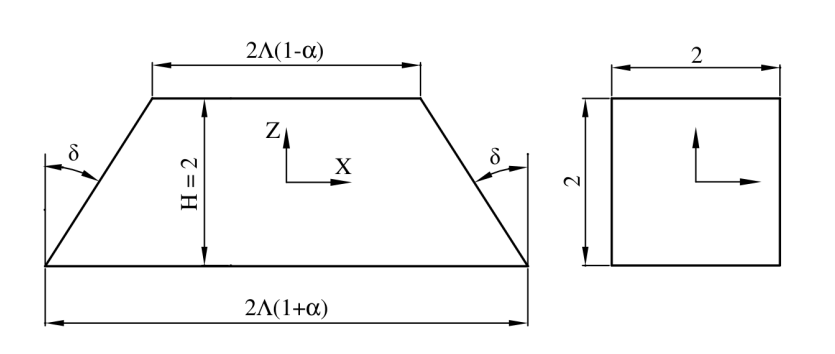
Consider a trapezoid and its interpolation into a reference space (square with side \(2\)).

The parametric space has coordinates \((\xi ,\zeta )\). The change in coordinates is written as:

\(\{\begin{array}{c}x=\mathrm{\Lambda }\xi (1-\alpha \zeta )\\ z=\zeta \end{array}\text{avec}\alpha \mathrm{\Lambda }=\mathrm{tan}(\delta )\) and \(\{\begin{array}{c}\xi =\frac{x}{\mathrm{\Lambda }(1-\alpha z)}\\ \zeta =z\end{array}\)

The Jacobian for change of coordinates is written as:

(1.12)\[ \begin{align}\begin{aligned}\begin{split} \ {\ begin {array} {c}\ frac {\ partial\ xi} {\ partial\ xi} {\ partial x} =\ frac {1} {\ mathrm {\ Lambda} (1-\ alpha\ zeta)}}\\ frac {\ frac {\ partial\ xi} {\ partial\ xi} =\ frac {\ alpha\ xi} {(1-\ alpha\ zeta)}\\ frac {\ partial\ xi} {\ partial z} =\ frac {\ alpha\ zeta)}\\ frac {\ partial\ xi} {\ partial z} =\ frac {\ alpha\ zeta)}\\ frac {\ partial\ xi} {\end{split}\\ \ textrm {and}\\\begin{split} \ {\ begin {array} {c}\ frac {\ partial\ zeta} {\ partial\ zeta} {\ partial x} =0\\ frac {\ partial\ zeta} {\ partial z} =1\ end {array}\end{split}\end{aligned}\end{align} \]

It will be noted that the Jacobian is not a constant step. If we assume for the sake of simplicity that \(\frac{M}{\mathit{EI}}=1\) and \(\nu =0\), the solution for moving a beam in pure bending is written as:

(1.13)\[\begin{split} \ {\ begin {array} {c} {u} ^ {u} ^ {\ mathit {beam}}} =xz\\ {w} ^ {\ mathit {beam}}} =-\ frac {1} {1} {2} {2} {2}\ end {array}} =-\ frac {1} {2} {2} {array}\end{split}\]

Or in the parametric space:

(1.14)\[\begin{split} \ {\ begin {array} {c} {u} ^ {u} ^ {\ mathit {beam}}} =\ mathrm {\ Lambda} (\ zeta\ xi -\ alpha\ xi {\ zeta} ^ {2})\\ {w}} ^ {2})\\ {w}} ^ {2} {\ mathrm {\ Lambda}} ^ {2})\\ {w}} ^ {2} ^ {2})\\ {w}} ^ {2} ^ {2} {2}\ left ({\ xi} ^ {2} + {\ alpha} + {\ alpha} ^ {2} {\ xi} ^ {2} {\ zeta} ^ {2} -2\ alpha\ zeta {\ xi} + {\ xi} + {\ alpha} ^ {2}\ right)\ end {array} -2\ alpha\ zeta {\ xi} -2\ alpha\ zeta {\ xi} ^ {xi} ^ {2}\ right)\ end {array}\end{split}\]

[Bib2] introduced the concept of aliasing interpolation functions into finite elements. The principle is as follows: in a finite element, we cannot approximate all the functions, everything will depend on the order of the polynomials used in these functions. For example, on a triangle with linear functions, we cannot represent quadratic functions. In the usual parametric representation, in 2D, we have the following table:

Element	TRIA3	QUAD4		TRIA6	QUAD8
Function
\({\xi }^{2}\)	\(\xi\)	\(1\)	\({\xi }^{2}\)	\({\xi }^{2}\)
\(\xi \eta\)	\(0\)	\(\xi \eta\)	\(\xi \eta\)	\(\xi \eta\)
\({\eta }^{2}\)	\(\eta\)	\(1\)	\({\eta }^{2}\)	\({\eta }^{2}\)
\({\xi }^{3}\)	\(\xi\)	\(\xi\)	\(\frac{1}{2}\left(3{\xi }^{2}-\xi \right)\)	\(\xi\)
\({\xi }^{2}\eta\)	\(0\)	\(\eta\)	\(\frac{1}{2}\xi \eta\)	\({\xi }^{2}\eta\)
\(\xi {\eta }^{2}\)	\(0\)	\(\xi\)	\(\frac{1}{2}\xi \eta\)	\(\xi {\eta }^{2}\)
\({\eta }^{3}\)	\(\eta\)	\(\eta\)	\(\frac{1}{2}\left(3{\eta }^{2}-\eta \right)\)	\(\eta\)
\({\xi }^{4}\)	\(\xi\)	\(1\)	\(\frac{1}{4}\left(7{\xi }^{2}-3\xi \right)\)	\({\xi }^{2}\)
\({\xi }^{3}\eta\)	\(0\)	\(\xi \eta\)	\(\frac{\xi \eta }{4}\)	\(\xi \eta\)
\({\xi }^{2}{\eta }^{2}\)	\(0\)	\(1\)	\(\frac{\xi \eta }{4}\)	\({\xi }^{2}+{\eta }^{2}-1\)
\({\xi }^{2}\eta\)	\(0\)	\(\xi \eta\)	\(\frac{\xi \eta }{4}\)	\(\xi \eta\)
\({\eta }^{4}\)	\(\eta\)	\(1\)	\(\frac{1}{4}\left(7{\eta }^{2}-3\eta \right)\)	\({\eta }^{2}\)

This array can be read as follows: for a function in \({\eta }^{3}\), an element TRIA3, QUAD4 or QUAD8 will represent, at best, the case \(\eta\) and for the TRIA6, we can represent by \(\frac{1}{2}\left(3{\eta }^{2}-\eta \right)\). Aliasing therefore transforms movements () as follows for QUAD4:

(1.15)\[ \ {\ begin {array} {c} {u} ^ {u} ^ {\ mathit {beam}} =\ mathrm {\ Lambda} (\ zeta\ xi -\ alpha\ xi {\ zeta} ^ {2})\ to {u} {2})\ to {u} ^ {2})\ to {u} ^ {^ {2})\ to {u} ^ {2})\ to {u} ^ {^ {2})\ to {u} ^ {^ {2})\ to {u} ^ {^ {2}) {\ mathit {EF}} =\ mathrm {\ Lambda} (\ zeta\ xi -\ zeta\ xi -\ zeta} {\ zeta} {\ zeta} ^ {2})\ to {u} ^ {\ mathit {beam}} =-\ frac {1} {1} {2} {\ mathrm {\ Lambda}} ^ {2}\ left ({\ xi} ^ {2} + {\ alpha} ^ {2} ^ {2} {\ xi} ^ {2} {\ xi} ^ {2}\ right)\ to {w} ^ {2}\ right)\ to {w} ^ {\ mathit {EF}} =-\ frac {1} {2} {2} {\ mathrm {\ Lambda}} ^ {2}\ left (1+ {\ alpha} ^ {2} -2\ alpha\ zeta\ right)\ end {array}\]

This results in the following deformations:

(1.16)\[ \begin{align}\begin{aligned} {\ epsilon} _ {\ mathit {xx}} =\ frac {\ partial u} {\ partial u} {\ partial x} =\ frac {\ partial\ xi}\ frac {\ partial\ xi} {\ partial\ xi} {\ partial x} {\ partial x} {\ partial x} {\ partial x} +\ frac {\ partial u} {\ partial u} {\ partial u} {\ partial u} {\ partial\ zeta}\ frac {\ partial x} =\ frac {\ partial x} =\ frac {\ partial x} =\ frac {\ partial x} =\ frac {\ partial x} =\ frac {\ partial x} =\ frac {\ partial x} =\ frac {\ partial x} =\ frac {\ partial x} = zeta -\ alpha} {1-\ alpha\ zeta}\\ {\ epsilon} _ {\ mathit {zz}} =\ frac {\ partial w} {\ partial w} =\ frac {\ partial w} {\ partial\ xi}\ frac {\ partial\ xi} {\ partial\ xi} {\ partial z} {\ partial z} {\ partial z} +\ frac {\ partial w} {\ partial w} {\ partial z} +\ frac {\ partial w} {\ partial w} {\ partial z} =\ frac {\ partial\ zeta} {\ partial z} =\ alpha {\ mama* thrm {\ Lambda}} ^ {2}\\\begin{split} {\ gamma} _ {\ mathit {xz}} =\ frac {1} {2}}\ left (\ frac {\ partial w} {\ partial x} +\ frac {\ partial u} {\ partial z}\ right) =\ mathrm {\ partial z}\\ right) =\ mathrm {\ Lambda}\ right) =\ mathrm {\ Lambda}\ xi\ left (1+\ frac {\ partial w} {\ partial x}} +\ frac {\ partial u} {\ partial u} {\ partial z}\ right) =\ mathrm {\ partial z}\ right) =\ mathrm {\ Lambda}\ right) =\ mathrm {\ Lambda}\ xi\ left (1+\ frac {\ partial zeta}\ right)\end{split}\end{aligned}\end{align} \]

However, the analytical solution (see ()) gives us:

\[\]

: label: eq-20

{begin {array} {c} {epsilon}} _ {mathit {xx}}} ^ {mathit {beam}} =z=zeta\ {epsilon} _ {mathit {zz}}} _ {mathit {zz}}} ^ {mathit {zz}}} ^ {mathit {zz}}} ^ {mathit {zz}}} ^ {mathit {zz}}} ^ {mathit {zz}}} ^ {mathit {zz}}} ^ {mathit {zz}}} ^ {mathit {zz}}} ^ {mathit {zz}}} ^ {mathit {zz}}} ^ {mathit {zz}}} ^ {mathit {zz}}} ^} =0end {array}

For contribution \({\epsilon }_{\mathit{xx}}\), the finite element solution is accurate for \(\alpha =0\) (perfect quadrangle) and the error remains small for a small \(\alpha\). The shear error \({\gamma }_{\mathit{xz}}\) can be canceled if we estimate the term in \((\mathrm{0,0})\). On the other hand, the term \({\epsilon }_{\mathit{zz}}\) has a bigger error than \({\gamma }_{\mathit{xz}}\) when it comes to \(\alpha \mathrm{\Lambda }=\mathrm{tan}\delta >1\). We therefore have a trapezoidal locking of the linear element as soon as we have edges that move away from the geometric case of the rectangle (or from the hexahedron for the 3D case).

1.1.5. Volume locking (incompressibility)

This type of locking is not specific to thin structures and occurs systematically when the material or behavior becomes incompressible, which generally corresponds to two situations:

• when the Poisson’s ratio tends to \(\mathrm{0,5}\), which is the case with hyperelastic materials such as elastomers for example;

• when the behavior is plastic, the plasticity of metals taking place at constant volume

It is a volume lock or incompressible. For the case of « massive » elements, there are several strategies to overcome this lockdown, see [R3.06.08] or [R3.06.14].

1.1.6. Methods to fix locks for COQUE_SOLIDE

To overcome these lockdowns, three ingredients are proposed:

To eliminate volume and membrane locking, we will use a**reduced integration* (RI) method which consists in using a less rich integration scheme than the one traditionally used for 8-node bricks. The reduced integration will cause parasitic modes with zero energy (or « hourglass » modes) to appear, which will be eliminated by a stabilization method;

To eliminate volume locking, an approach based on incompatible modes is also proposed in its generic formulation called « * EAS ** » (Enhanced Assumed Strain) which will enrich the approximation to correct the pinching problem;

To eliminate transverse and trapezoidal shear locking, the assumed field method (* ANS ** « Assumed Natural Strain ») will be used.

The EAS (Enhanced Assumed Strain) method, whose formalism is based on Hu-Washizu’s three-field formulation, was initially proposed by [Bib2, Bib3] in small deformations, then extended to large deformations by [Bib4,Bib5] before being applied to thermomechanical problems by [Bib6]. This method is a generalization of the method of incompatible modes. It consists in reducing the order of the polynomials for certain components of the deformations.

This method makes it possible to significantly reduce volume locking. Recent work [Bib8], [Bib9] has shown that a single parameter is sufficient, which also makes it possible to be consistent with reduced integration. However, in certain configurations (compression loading), instabilities appear, and it is also necessary in the case of plate elements to overcome transverse shear interlocks. We are going to combine method EAS with method ANS and taking into account the pinch.

Technique ANS (« Assumed Natural Strain ») consists in replacing the transverse shear deformation by a postulated shear deformation obtained by interpolation into the natural base of the element (hence the qualifier « natural »). In addition to facilitating the management of shear locking, interpolation into the natural base results in elements operating with a more or less deformed mesh.