2. Formulation#
2.1. Geometry#
For eccentric plate elements, the reference surface is given by the draft plane or mesh plane (plane \(xy\) for example). The middle sheet of the element is positioned in relation to this reference surface. Thickness \(h(x,y)\) must be small compared to the other dimensions (extensions, radii of curvature) of the structure to be modelled. Figure [Figure 2.1-a] below illustrates our point. Regarding the value of the eccentricity \(d\), and because of the conditions for linearization of the flexure adopted in the theory, \(d\) will be taken so that an element of thickness \(d+h\) remains in the theory of plates.
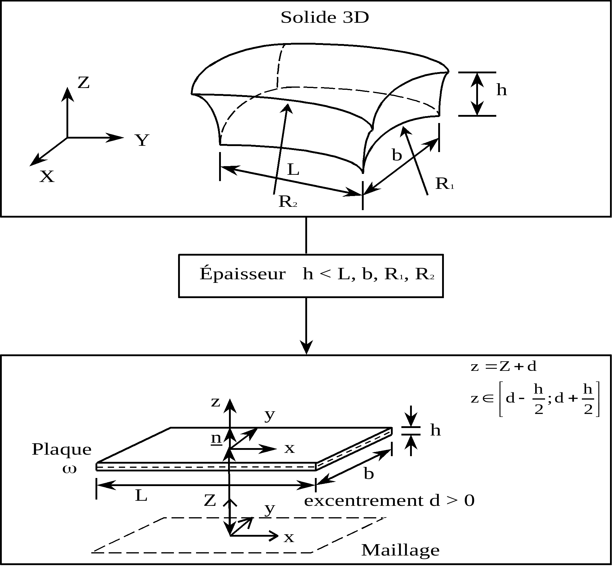
Figure 2.1-a
A local orthonormal coordinate system \(\mathrm{0xyz}\) associated with the mesh plane different from the global coordinate system \(\mathit{OXYZ}\) is attached to the design plane (the mesh plane). The position of the points on the plate is given by the Cartesian coordinates \((x,y)\) in the drawing plane (mesh plane) and the elevation \(z\) with respect to this plane.
2.2. Cinematics#
The straight sections, which are the sections perpendicular to the middle sheet of the plate, remain straight. The material points located on a normal to the undeformed mean surface remain on a line in the deformed configuration. As a result of this approach, the displacement fields vary linearly in the thickness of the plate. If we designate by \(u,v,w\) the movements of a point in the drawing plane \(q(x,y,z)\) following \(x\), \(y\) and \(z\), the Hencky-Mindlin kinematics gives us:
\((\begin{array}{c}{u}_{x}(x,y,z)\\ {u}_{y}(x,y,z)\\ {u}_{z}(x,y,z)\end{array})=(\begin{array}{c}u(x,y)\\ v(x,y)\\ w(x,y)\end{array})+z(\begin{array}{c}{\theta }_{y}(x,y)\\ -{\theta }_{x}(x,y)\\ 0\end{array})=(\begin{array}{c}u(x,y)\\ v(x,y)\\ w(x,y)\end{array})+z(\begin{array}{c}{\beta }_{x}(x,y)\\ {\beta }_{y}(x,y)\\ 0\end{array})\)
where: |
\(u,v,w\) are the movements of the draft plane; |
\({\theta }_{x}\) and \({\theta }_{y}\) are respectively the rotations of this plane with respect to the axis \(x\) and the axis \(y\) respectively. |
It is preferred to introduce the two \({\beta }_{x}(x,y)\mathrm{=}{\theta }_{y}(x,y),{\beta }_{y}(x,y)\mathrm{=}\mathrm{-}{\theta }_{x}(x,y)\) rotations. The three-dimensional deformations at any point, with the kinematics introduced earlier, are thus given by:
\(\begin{array}{}{\epsilon }_{\text{xx}}={e}_{\text{xx}}+{\mathrm{z\kappa }}_{\text{xx}}\\ {\epsilon }_{\text{yy}}={e}_{\text{yy}}+{\mathrm{z\kappa }}_{\text{yy}}\\ {\mathrm{2\epsilon }}_{\text{xy}}={\gamma }_{\text{xy}}=2{e}_{\text{xy}}+{\mathrm{2z\kappa }}_{\text{xy}}\\ {\mathrm{2\epsilon }}_{\text{xz}}={\gamma }_{x}\\ {\mathrm{2\epsilon }}_{\text{yz}}={\gamma }_{y}\end{array}\)
where: |
\({e}_{\mathit{xx}}\), \({e}_{\mathit{yy}}\) and \({e}_{\mathit{xy}}\) are the mean surface membrane strains; \({\gamma }_{x}\) and \({\gamma }_{y}\) the deformations associated with transverse shears; \({\kappa }_{\mathit{xx}}\), \({\kappa }_{\mathit{yy}}\), \({\kappa }_{\mathit{xy}}\) the flexural deformations of the mean surface, which are written as: |
\(\begin{array}{}{e}_{\text{xx}}=\frac{\partial u}{\partial x}\\ {e}_{\text{yy}}=\frac{\partial v}{\partial y}\\ 2{e}_{\text{xy}}=\frac{\partial v}{\partial x}+\frac{\partial u}{\partial y}\\ {\kappa }_{\text{xx}}=\frac{\partial {\beta }_{x}}{\partial x}\\ {\kappa }_{\text{yy}}=\frac{\partial {\beta }_{y}}{\partial y}\\ {\mathrm{2\kappa }}_{\text{xy}}=\frac{\partial {\beta }_{x}}{\partial y}+\frac{\partial {\beta }_{y}}{\partial x}\\ {\gamma }_{x}={\beta }_{x}+\frac{\partial w}{\partial x}\\ {\gamma }_{y}={\beta }_{y}+\frac{\partial w}{\partial y}\end{array}\)
Note:
In plate theories, the introduction of \({\beta }_{x}\) and \({\beta }_{y}\) makes it possible to symmetrize deformation formulations and equilibrium equations [R3.07.03]. In shell theories, we instead use \({\theta }_{x}\) and \({\theta }_{y}\) and the associated couples \({M}_{x}\) and \({M}_{y}\) versus \(x\) and \(y\) ,
the degrees of freedom that we have chosen are the movements and rotations of the design plane and not those of the middle sheet. In fact, if one considers the superposition of several eccentric plates to produce a sandwich material, only one field of displacement can correspond to the nodes of the mesh and not to the various fields of movement of the layers composing the material.
2.3. Law of behavior#
The behavior of the plates is a 3D behavior under « plane stresses ». The transverse constraint \({\sigma }_{\mathit{zz}}\) is taken to be zero because it is negligible compared to the other components of the stress tensor (plane stress hypothesis). The most general law of behavior is then written as follows:
\((\begin{array}{c}{\sigma }_{\text{xx}}\\ {\sigma }_{\text{yy}}\\ {\sigma }_{\text{xy}}\\ {\sigma }_{\text{xz}}\\ {\sigma }_{\text{yz}}\end{array})=C(\epsilon ,\alpha )(\begin{array}{c}{\epsilon }_{\text{xx}}\\ {\epsilon }_{\text{yy}}\\ {\gamma }_{\text{xy}}\\ {\gamma }_{x}\\ {\gamma }_{y}\end{array})=\text{Ce}+\mathrm{zC\kappa }+\mathrm{C\gamma }\) with \(e=\left(\begin{array}{c}{e}_{\text{xx}}\\ {e}_{\text{yy}}\\ 2{e}_{\text{xy}}\\ 0\\ 0\end{array}\right),\text{}\kappa =\left(\begin{array}{c}{\kappa }_{\text{xx}}\\ {\kappa }_{\text{yy}}\\ 2{\kappa }_{\text{xy}}\\ 0\\ 0\end{array}\right)\phantom{\rule{0.5em}{0ex}}\text{et}\phantom{\rule{0.5em}{0ex}}\gamma =\left(\begin{array}{c}0\\ 0\\ 0\\ {\gamma }_{x}\\ {\gamma }_{y}\end{array}\right)\)
where: \(C(\varepsilon ,\alpha )\) is the local tangent stiffness matrix in plane stresses;
\(\alpha\) represents the set of internal variables when the behavior is non-linear.
For behaviors (for example multilayers) for which the distortions are coupled to membrane and flexural deformations, \(C(\varepsilon ,\alpha )\) takes the form:
\(C\mathrm{=}(\begin{array}{cc}H& {H}_{c\gamma }\\ {H}_{{c\gamma }_{}}^{T}& {H}_{\gamma }\end{array})\)
where: |
\(H(\varepsilon ,\alpha )\) is a symmetric \(3\mathrm{\times }3\) matrix; \({H}_{\gamma }(\varepsilon ,\alpha )\) a symmetric \(2\mathrm{\times }2\) matrix; \({H}_{c\gamma }(\varepsilon ,\alpha )\) a \(3\mathrm{\times }2\) matrix for coupling between membrane effects or flexure and transverse shear effects. |
In case it is decoupled, we have \({H}_{c\gamma }(\varepsilon ,\alpha )\mathrm{=}0\). The determination of \({H}_{\gamma }(\varepsilon ,\alpha )\) in the framework of Reissner’s theory ([§2.2.3.2] of [R3.07.03]) is given in the appendix. It is shown that it is equivalent to that of the non-eccentric plates.