2. Formulation#
2.1. Shell geometry#
For the solid shell elements \(\Omega\), a reference surface \(\omega\), or average, left surface is defined (with curvilinear coordinates \({\xi }_{1}{\xi }_{2}\) for example) and a thickness \(h({\xi }_{1}{\xi }_{2})\) measured according to the normal to the average surface. This thickness must be small compared to the other dimensions (extensions, radii of curvature) of the structure to be modelled. Figure [Figure 2.1-a] below illustrates our point.
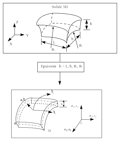
Figure 2.1-a
The position of the points on the shell is given by the curvilinear coordinates \(({\xi }_{1}{\xi }_{2})\) of the mean surface \(\omega\) and the elevation \({\xi }_{3}\) with respect to this surface. \((O,{e}_{k})\) is the global Cartesian coordinate system, with associated axes \(({x}_{k})\).
2.1.1. Geometric description of the mean surface#
Local natural base and local Cartesian basis
Let \(P\) be any point on the mean reference surface \(\omega\), we have:
\(\text{OP}\mathrm{=}{x}_{k}^{0}({\xi }_{1},{\xi }_{2}){e}_{k}\)
We define the vectors \({a}_{\alpha }\) of the natural local base of the tangential plane in \(P\) to \(\omega\), attached to \(P\) by:
\({a}_{\alpha }\mathrm{=}\frac{\mathrm{\partial }\text{OP}}{\mathrm{\partial }{\xi }_{\alpha }}\mathrm{=}{\text{OP}}_{,\alpha }\)
and we define the unit normal \(n\) by:
\(n\mathrm{=}\frac{{a}_{1}\mathrm{\wedge }{a}_{2}}{\mathrm{\parallel }{a}_{1}\mathrm{\wedge }{a}_{2}\mathrm{\parallel }}\)
\({\xi }_{3}\) is the position variable in the thickness associated with \(n\).
\(\left({a}_{1},{a}_{2},{a}_{3}\right)\) is the natural base attached to \(P\).
The curvilinear coordinate system \(({\xi }_{1}{\xi }_{2})\) is not necessarily orthogonal, so the base \(({a}_{\alpha })\) is not necessarily orthogonal (and even less orthonormal). An orthonormal local base \({t}_{k}\) is therefore defined as follows:
\({t}_{1}\mathrm{=}\frac{{a}_{1}}{\mathrm{\parallel }{a}_{1}\mathrm{\parallel }},{t}_{2}\mathrm{=}n\mathrm{\wedge }{t}_{1}{t}_{3}\mathrm{=}n\)
and we note \(\left({s}_{1},{s}_{2}\right)\) the coordinate system associated with \(\left({t}_{1},{t}_{2}\right)\).
Intrinsic reference
The local base \({t}_{k}\) will be used to define the intrinsic coordinate system of a shell element by choosing as point P the first vertex of the element and for vector \({a}_{1}\) a vector coinciding with the projection of the first side on the tangential plane at the first vertex.
Curvature tensor calculation
The curvature tensor is related to the change in the normal on \(\omega\). It is defined by its mixed components:
\({n}_{,\beta }\text{=-}{C}_{\beta }^{\gamma }{a}_{\gamma }\)
or by its covariant components: \({C}_{\alpha \beta }\text{=-}{a}_{\alpha }\text{.}{n}_{,\beta }\mathrm{=}n\text{.}{a}_{\alpha ,\beta }\). This tensor is symmetric since \({a}_{\alpha ,\beta }\mathrm{=}{a}_{\beta ,\alpha }\). Its track \(\text{tr}{C}_{\alpha \beta }\) is the mean curvature and its determinant the Gaussian curvature.
2.1.2. Description of the geometry of the shell#
Let \(Q\) be any point in \(\Omega\), volume of the shell whose thickness \(h\) is considered constant, we have:
\(\text{OQ}+\text{OP}+\text{PQ}\mathrm{=}\text{OP}+\frac{{\xi }_{3}}{2}hn\)
where \({\xi }_{3}\mathrm{\in }\left[\mathrm{-}\mathrm{1,1}\right]\).
\(({\xi }_{1},{\xi }_{2},\frac{{\xi }_{3}}{2}h)\) is a curvilinear coordinate system of \(\Omega\).
We can also write \(\text{OQ}\) in terms of its \(({x}_{k})\) components in the global base \(({e}_{k})\):
\(\text{OQ}\mathrm{=}{x}_{k}{e}_{k}\)
Local natural base, local orthonormal base and metric tensor
As with \(P\), we define the natural base of the 3D space \(({g}_{k})\) attached to \(Q\) by:
\({g}_{\alpha }\mathrm{=}\frac{\mathrm{\partial }\text{OQ}}{\mathrm{\partial }{\xi }_{\alpha }}\mathrm{=}{a}_{\alpha }+{\xi }_{3}\frac{h}{2}{n}_{,\alpha },{g}_{3}\mathrm{=}\frac{{g}_{1}\mathrm{\wedge }{g}_{2}}{\mathrm{\parallel }{g}_{1}\mathrm{\wedge }{g}_{2}\mathrm{\parallel }}\mathrm{=}n\)
Since \(({g}_{k})\) is not necessarily orthogonal, an orthonormal local base \(({T}_{k})\) is defined as follows:
\({T}_{1}\mathrm{=}\frac{{g}_{1}}{\mathrm{\parallel }{g}_{1}\mathrm{\parallel }},{T}_{2}\mathrm{=}n\mathrm{\wedge }{T}_{1},{T}_{3}\mathrm{=}n\)
and we note \(({x}_{k})\) the coordinate system associated with \(({T}_{k})\).
We’ll call \(({T}_{k})\) the local orthonormal base, and \(({x}_{k})\) the coordinates in this local orthonormal base.
By definition, we have:
\({T}_{k}\mathrm{=}\frac{\mathrm{\partial }\text{OQ}}{\mathrm{\partial }{\tilde{x}}_{k}}\mathrm{=}\frac{\mathrm{\partial }{x}_{j}}{\mathrm{\partial }{\tilde{x}}_{k}}{e}_{j}\mathrm{=}{T}_{k}^{j}{e}_{j}\)
with \(\frac{\mathrm{\partial }{x}_{j}}{\mathrm{\partial }{\tilde{x}}_{k}}\mathrm{=}{T}_{k}^{j}\) the components of \(({T}_{k})\) in the global \(({e}_{j})\) base. (These are also the components of the transition matrix from \(({T}_{k})\) to \(({e}_{j})\) since the transition matrix is orthogonal. So if \({T}_{k}={T}_{k}^{j}{e}_{j}\) we also have \({e}_{k}={T}_{j}^{k}{T}_{j}\)).
The metric tensor \(G\) associated with \(Q\) is defined by its components deduced from the dot products of the vectors of the local orthonormal base:
\({G}_{\text{ij}}={T}_{i}\text{.}{T}_{j}\)
This \(G\) tensor is equivalent to the \(\text{Id}\) identity.
2.1.3. note#
Figures [Figure 2.1.3-a] and [Figure 2.1.3-b] illustrate the geometric quantities mentioned above.
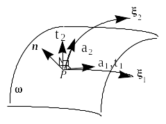
Figure 2.1.3-a
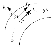
Figure 2.1.3-b
It should be noted that the two local orthonormal bases, the one associated with the mean surface \(({t}_{k})\) and the other with the volume of the shell \(({T}_{k})\), are only combined when the curvature is zero. In this case, the shell elements are similar to plate elements.
2.2. Plate and shell theory#
These elements are based on the theory of plates and shells according to which:
2.2.1. Cinematics#
2.2.1.1. Travel field#
Straight sections that are sections perpendicular to the mean surface remain straight; material points located on a normal to the undeformed mean surface remain on a line in the deformed configuration. As a result of this approach, displacement fields vary linearly in shell thickness.
If we write \(Q\text{'}\), the position of \(Q\) after deformation, we have:
\(\text{OQ}\text{'}\mathrm{=}\text{OQ}+\text{QQ}\text{'}\mathrm{=}\text{OQ}+U(Q)\)
where the chosen displacement field, corresponding to the Hencky-Mindlin kinematics, is written:
\(U(Q)\mathrm{=}u(P)+\frac{{\xi }_{3}}{2}h\beta (P)\) with \(\beta (P)\text{.}n\mathrm{=}0\)
where \(u(P)\) and \(\beta (P)\) are respectively the displacement vector and the rotation vector of \(P\), projection of \(Q\) on the mean surface of the shell. The fact that \(\beta (P)\text{.}n\mathrm{=}0\) indicates that the rotations of the shell around its normal are not taken into account in this kinematics.
Rating:
We denote \(\stackrel{}{˜}\) the quantities expressed in the local Cartesian bases \(({t}_{k})\) or \(({T}_{k})\) for the points \(P\) and \(Q\) respectively. The result is that:
the three-dimensional displacement vector \(U\) can be written \(U\mathrm{=}{\tilde{U}}_{k}{T}_{k}\) or even \(U\mathrm{=}{U}_{k}{e}_{k}\), where it is expressed respectively in its local orthonormal base or in the global Cartesian base,
the displacement vector of the mean surface \(u\) can be written \(u\mathrm{=}{\tilde{u}}_{k}{t}_{k}\) or \(u\mathrm{=}{u}_{k}{e}_{k}\) depending on whether it is expressed in its local orthonormal base or in the global Cartesian base,
The mean surface rotation vector is written \(b\mathrm{=}{\tilde{\beta }}_{\alpha }{t}_{\alpha }\) in its local orthornormed base. \(\beta\) being the rotation of the normal \(\mathrm{n}\) (at the mean surface), we also write \(\beta \mathrm{=}\theta \mathrm{\wedge }n\) with \(\theta\), the rotation vector of the mean surface, such as \(\theta \mathrm{=}{\tilde{\theta }}_{\alpha }{t}_{\alpha }\). The equivalence of the two formulations shows that \({\tilde{\beta }}_{1}\mathrm{=}{\tilde{\theta }}_{2},{\tilde{\beta }}_{2}\mathrm{=}\mathrm{-}{\tilde{\theta }}_{1}\).
2.2.1.2. Expression of three-dimensional deformations#
The deformation tensor is calculated in the local orthonormal Cartesian base \(({T}_{k})\). It is defined as the half-difference of the metric tensors associated with the local orthonormal bases after and before deformation. The metric tensor associated with this base in the undeformed state is simply identity \(\text{Id}\), while the metric tensor for the deformed state is \({\overline{G}}_{\text{ij}}\mathrm{=}{T}_{i}\text{'}\text{.}T{\text{'}}_{j}\) with \(T{\text{'}}_{k}\mathrm{=}\frac{\mathrm{\partial }\text{OQ}\text{'}}{\mathrm{\partial }{\tilde{x}}_{k}}\).
The components of the strain tensor in \(({T}_{k})\) are thus given by:
\(\begin{array}{c}{\tilde{e}}_{\text{αβ}}\mathrm{=}\frac{1}{2}(\frac{\P {\tilde{U}}_{\alpha }}{\P {\tilde{x}}_{\beta }}+\frac{\P {\tilde{U}}_{\beta }}{\P {\tilde{x}}_{\alpha }})\\ {\tilde{e}}_{\mathit{\alpha 3}}\mathrm{=}\frac{1}{2}(\frac{\P {\tilde{U}}_{\alpha }}{\P {\tilde{x}}_{3}}+\frac{\P {\tilde{U}}_{3}}{\P {\tilde{x}}_{\alpha }})\end{array}\)
The equations above are linear deformation-displacement relationships. Displacement variables are the \({\tilde{U}}_{k}\) component.
The components \({\tilde{\varepsilon }}_{\text{kl}}\) of the \(\tilde{\varepsilon }\) tensor can also be expressed as a function of the components in the global coordinate system \(\frac{\mathrm{\partial }{U}_{p}}{\mathrm{\partial }{x}_{m}}\). In fact, as in the global coordinate system \(\varepsilon \mathrm{=}{\varepsilon }_{\text{ij}}{e}^{i}\mathrm{\times }{e}^{j}\mathrm{=}{\varepsilon }_{\text{ij}}{T}_{k}^{i}{T}_{l}^{j}{T}^{k}\mathrm{\times }{T}^{l}\mathrm{=}{\tilde{\varepsilon }}_{\text{kl}}{T}^{k}\mathrm{\times }{T}^{l}\), we therefore immediately deduce that: \({\tilde{\varepsilon }}_{\text{kl}}\mathrm{=}{\varepsilon }_{\text{ij}}{T}_{k}^{i}{T}_{l}^{j}\). \(({e}^{k})\) and \(({T}^{k})\) are the contravariant bases associated with \(({e}_{k})\) and \(({T}_{k})\) respectively such as: \({e}^{i}\text{.}{e}_{j}\mathrm{=}{\delta }_{\text{ij}}\) and. \({T}^{i}\text{.}{T}_{j}\mathrm{=}{\delta }_{\text{ij}}\) As the bases \(({e}_{k})\) and \(({T}_{k})\) are orthonormal, their associated contravariant bases are confused with themselves. So in the same way that we had \({T}_{k}\mathrm{=}{T}_{k}^{j}{e}_{j}\) we find \({T}^{k}={T}_{k}^{j}{e}^{j}\) again.
If we write down \(T\mathrm{=}{T}_{k}^{i}{e}_{i}\mathrm{\times }{T}^{k}\) then \(T\mathrm{\times }T\mathrm{:}\varepsilon \mathrm{=}{\tilde{\varepsilon }}_{\text{kl}}{T}^{k}\mathrm{\times }{T}^{l}\mathrm{=}\tilde{\varepsilon }\). Hereinafter, \(\tilde{\varepsilon }\) designates the expression for the deformations tensor in the local orthonormal coordinate system and \(\varepsilon\) designates the expression of the same tensor in the global coordinate system. The transition relationship from one to the other is given above in terms of tensors.
Notes:
The terms \({T}_{k}^{j}\) contain shell curvature terms \(\Omega\) .
We note in the deformation-displacement relationships that the component \({\tilde{\varepsilon }}_{\text{33}}\) is not determined by kinematics. This is associated with the hypothesis of the nullity of normal transverse constraints \({\tilde{\sigma }}_{\text{33}}\mathrm{=}0\) justified by the behavior of the shells.
In the literature (see for example [bib3]), the modeling of shells by the approach based on the \({\tilde{u}}_{k}\) curvilinear components of the displacement explicitly reveals the curvature quantities at the level of the expression of the deformation tensor [bib5]. As, in general, the geometry of the shell is not explicitly known, it is therefore necessary to determine numerically the geometric characteristics that are the vectors \({a}_{\alpha },{g}_{\alpha }\) ,… and the curvatures \({C}_{\alpha \beta }\). With the finite element method it is necessary to derive the shape functions twice (see page 20 of [bib5] and [R3.07.02]) to calculate the \({C}_{\alpha \beta }\) . This may make their calculation inaccurate depending on the family of form functions chosen. The error committed depends on these (linear, quadratic, cubic polynomials…) and becomes independent of the refinement of the mesh. A formulation involving the first derivation of shape functions (calculation of slopes) does not have this disadvantage. Thus, the error resulting from the calculations of curvature terms in a formulation based on the curvilinear approach does not decrease with the refinement of the mesh, whereas for the formulation described above it becomes small by increasing the number of finite elements. In view of the previous observations, the so-called curvilinear approach was not followed.
2.2.2. Law of behavior#
The behavior of shells is a 3D behavior under « plane constraints ». It links the components of stresses and strains, in the form of vectors, in the local orthonormal base. The transverse stress \({\tilde{\sigma }}_{\text{33}}\) is zero because it is considered to be negligible compared to the other components of the stress tensor (plane stress hypothesis). The most general law of behavior is then written as follows:
\((\begin{array}{c}{\tilde{\sigma }}_{\text{11}}\\ {\tilde{\sigma }}_{\text{22}}\\ {\tilde{\sigma }}_{\text{12}}\\ {\tilde{\sigma }}_{\text{13}}\\ {\tilde{\sigma }}_{\text{23}}\end{array})\mathrm{=}\tilde{C}(\varepsilon ,\mu )(\begin{array}{c}{\tilde{\varepsilon }}_{\text{11}}\mathrm{-}{\tilde{\varepsilon }}_{\text{11}}^{\text{th}}\\ {\tilde{\varepsilon }}_{\text{22}}\mathrm{-}{\tilde{\varepsilon }}_{\text{22}}^{\text{th}}\\ {\tilde{\gamma }}_{\text{12}}\\ {\tilde{\gamma }}_{1}\\ {\tilde{\gamma }}_{2}\end{array})\)
where \(\tilde{C}(\varepsilon ,\mu )\) is the local behavior matrix under plane constraints and \(\mu\) represents all the internal variables when the behavior is non-linear.
For behaviors where transverse distortions are decoupled from membrane and flexural deformations, \(\tilde{C}(\varepsilon ,\mu )\) takes the form:
\(\tilde{C}\mathrm{=}(\begin{array}{cc}\tilde{H}& 0\\ 0& {\tilde{H}}_{\gamma }\end{array})\)
where \(\tilde{H}(\varepsilon ,\mu )\) is a membrane-bending behavior matrix \(3\mathrm{\times }3\) and \({\tilde{H}}_{\gamma }(\varepsilon ,\mu )\) is a matrix of transverse distortion behavior \(2\mathrm{\times }2\). Since the two phenomena are decoupled, we can also write the behavior in the form:
\((\begin{array}{c}{\tilde{\sigma }}_{\text{mf}}\\ {\tilde{\sigma }}_{g}\end{array})\mathrm{=}\tilde{C}(\varepsilon ,\mu )(\begin{array}{c}{\tilde{\varepsilon }}_{\text{mf}}\\ \tilde{\gamma }\end{array})\) with:
\({\tilde{\sigma }}_{\text{mf}}\mathrm{=}(\begin{array}{c}{\tilde{\sigma }}_{\text{11}}\\ {\tilde{\sigma }}_{\text{22}}\\ {\tilde{\sigma }}_{\text{12}}\end{array})\mathrm{=}\tilde{H}(\varepsilon ,\mu )(\begin{array}{c}{\tilde{\varepsilon }}_{\text{11}}\mathrm{-}{\tilde{\varepsilon }}_{\text{11}}^{\text{th}}\\ {\tilde{\varepsilon }}_{\text{22}}\mathrm{-}{\tilde{\varepsilon }}_{\text{22}}^{\text{th}}\\ {\tilde{\gamma }}_{\text{12}}\end{array})\mathrm{=}\tilde{H}(\varepsilon ,\mu ){\tilde{\varepsilon }}_{\text{mf}}\) and \({\tilde{\sigma }}_{\gamma }\mathrm{=}(\begin{array}{c}{\tilde{\sigma }}_{\text{13}}\\ {\tilde{\sigma }}_{\text{23}}\end{array})\mathrm{=}{\tilde{H}}_{\gamma }(\varepsilon ,\mu )(\begin{array}{c}{\tilde{\gamma }}_{1}\\ {\tilde{\gamma }}_{2}\end{array})\mathrm{=}{\tilde{H}}_{\gamma }(\varepsilon ,\mu )\tilde{\gamma }\)
From now on, we will remain within the framework of this hypothesis.
For an isotropic homogeneous linear elastic behavior, we thus have:
\(\tilde{C}\mathrm{=}\frac{E}{1\mathrm{-}{\nu }^{2}}(\begin{array}{ccccc}1& \nu & 0& 0& 0\\ \nu & 1& 0& 0& 0\\ 0& 0& \frac{1\mathrm{-}\nu }{2}& 0& 0\\ 0& 0& 0& \frac{k(1\mathrm{-}\nu )}{2}& 0\\ 0& 0& 0& 0& \frac{k(1\mathrm{-}\nu )}{2}\end{array})\)
where \(k\) is a transverse shear correction factor whose meaning is given in the plate element reference documentation [R3.07.03], and [bib4] for more details. This coefficient is equal to \(5\mathrm{/}6\) for a Reissner-type theory and \(1\) for the Hencky—Mindlin theory. Finally, if we choose \(k\) very big, we are back to a Love-Kirchhoff theory. The transverse distortion is neutralized by penalizing the associated energy by taking \(k\mathrm{=}{10}^{6}h\mathrm{/}R\) (\(h\) being the thickness of the shell and \(R\) its mean radius of curvature).
Also in the isotropic case, the only two non-zero components of \({\tilde{\varepsilon }}^{\text{th}}\) are \({\tilde{\varepsilon }}_{\text{ii}}^{\text{th}}\) for \(i\mathrm{=}\mathrm{1,2}\), such that:
\({\tilde{\varepsilon }}_{\text{ii}}^{\text{th}}\mathrm{=}\alpha (T\mathrm{-}{T}^{\mathit{réf}})\)
where \(\alpha\) is the thermal expansion coefficient and \(T\mathrm{-}{T}^{\mathit{réf}}\) is the temperature difference that is assumed to be known.
Note:
We do not describe the variation in thickness or that of the transverse deformation \({\tilde{e}}_{\text{33}}\) which can however be calculated using the previous hypothesis of plane stresses. Moreover, no restriction is made on the type of behavior under plane constraints that can be represented.
In the same way as \(T\mathrm{\times }T\mathrm{:}\varepsilon \mathrm{=}\tilde{\varepsilon }\) we can deduce \((T\mathrm{\times }T{)}_{\text{mf}}\mathrm{:}\varepsilon \mathrm{=}{T}_{\text{mf}}\mathrm{:}\varepsilon \mathrm{=}{\tilde{\varepsilon }}_{\text{mf}}\) and \((T\mathrm{\times }T{)}_{\gamma }\mathrm{:}\varepsilon \mathrm{=}{T}_{\gamma }\mathrm{:}\varepsilon \mathrm{=}{\tilde{\varepsilon }}_{\gamma }\) , which makes it possible to find \({\tilde{\varepsilon }}_{\text{mf}}\) and \({\tilde{\varepsilon }}_{\gamma }\) from the tensor of the deformations in the global coordinate system.