3. Cohesive law integration CZM_TAC_MIX#
Cohesive behavior is determined by the density of cohesive energy \(\Pi (\delta )\). Although the variational formulation presented in the previous part is independent of the choice of cohesive energy, we are now interested in a particular cohesive model whose specificities are detailed. These main characteristics are:
contact conditions (non-interpenetration of the lips);
perfect initial adhesion (no regulation of surface energy);
coupling between failure modes (traction and shear);
total rupture, (zero cohesive forces beyond a certain damage threshold);
irreversibility of the rupture.
In particular, this means that there is no final friction, nor is there any distinction between tensile and shear failure mechanisms.
**Note:*
The Code_Aster keyword corresponding to this cohesive law is CZM_TAC_MIX. For more details on this law (internal variables, input parameters, coherent tangent matrix) and on other cohesive laws, we can refer to 5 (R7.02.11) .
3.1. Preliminary notations#
Because of the non-interpenetrating stress of the crack lips, the normal \(n\) direction for the surface of potential discontinuity \(\Gamma\) (opening/compression) must be distinguished from the directions in the plane (sliding, shear). To do this, the following notations are introduced, where \(v\) represents any vector quantity:
\({v}_{n}=v\cdot n;{v}_{\text{//}}=v-{v}_{n}n;{\langle v\rangle }_{+}=\langle {v}_{n}\rangle n+{v}_{\text{//}};{\parallel v\parallel }_{+}={({\langle v\rangle }_{+}\cdot {\langle v\rangle }_{+})}^{1/2}\)
and where \(\langle \text{.}\rangle\) refers to the positive part of a scalar.
3.2. Definition of cohesive law#
The cohesive law proposed by Talon and Curnier 5 meets the five points mentioned above and falls within the framework of energy formulation. The responses of the model subjected to pure tension and pure shear, as well as the stress initiation criterion are detailed Figure 3.2-a.
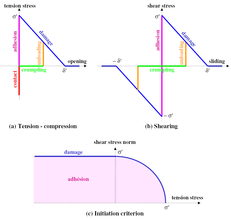
Figure 3.2-a : Talon Curnier law answers CZM_TAC_MIX in pure tension-compression (a), pure shear (b) and stress initiation criterion (c)
The corresponding cohesive energy is defined as follows:
First, the displacement discontinuities in opening and in shear are combined in a single scalar \({\delta }_{\text{eq}}\) which measures the magnitude of the discontinuity, thus responding to point 3:
\({\delta }_{\text{eq}}=N(\delta )=\sqrt{\delta \cdot \delta }\)
Then, irreversibility 3 is taken into account via a new scalar internal variable \(\kappa\) which measures the current maximum load level:
\(\kappa (t)=\underset{{t}^{\text{'}}<t}{\text{max}}{\delta }_{\text{eq}}({t}^{\text{'}})\)
The cohesive energy depends on the internal variable \(\kappa\) and the equivalent displacement jump \({\delta }_{\text{eq}}\). Contact conditions 3 are managed by an indicator function that imposes a positive normal discontinuity \({\delta }_{n}\ge 0\):
\(\Pi (\delta ,\kappa )={I}_{{ℝ}^{+}}({\delta }_{n})+\psi (\text{max}({\delta }_{\text{eq}},\kappa ))\)
In particular, function \(\psi\) characterizes the reaction to a load in pure I mode. According to 5, \(\psi\) must be an increasing and differentiable function, where \({\sigma }^{c}={\psi }^{\text{'}}(0)\) defines the critical constraint, a parameter of the priming criterion 3 represented on the Figure 3.2-a. In addition, the stability of the rupture process requires \(\psi\) to be concave 5. Finally, the final break 3 occurs as soon as \(\psi\) reaches its upper limit \({G}^{c}\) for a finite value \({\delta }_{\text{eq}}={\delta }^{c}\), where \({G}^{c}\) is the rupture energy and \({\delta }^{c}\) the critical opening beyond which the cohesive forces cancel each other out.
Thus, we choose the following function \(\psi\) which corresponds to the answers represented on Figure 3.2-a:
\(\psi ({\delta }_{\text{eq}})=\{\begin{array}{cc}{G}^{c}\frac{{\delta }_{\text{eq}}}{{\delta }^{c}}(2-\frac{{\delta }_{\text{eq}}}{{\delta }^{c}})& \text{if}{\delta }_{\text{eq}}\le {\delta }^{c}\\ {G}^{c}& \text{if}{\delta }_{\text{eq}}\ge {\delta }^{c}\end{array}\)
with the relationship between material parameters;
\({G}^{c}=\frac{1}{2}{\sigma }^{c}{\delta }^{c}\)
At this stage, the energy and the cohesive law derived from it are fully defined. However, one can explicitly express the relationship between displacement discontinuity \(\delta\) and the stress vector \(t\), condensed in the following differential inclusion, where \(\partial \Pi\) is the subdifferential of \(\Pi\) (see Clarke 5):
\(t\in \partial \Pi (\delta )\)
For a given value of \(\kappa\), we can interpret the sub-differential \(\partial \Pi (\delta )\) as the cone formed by the set of slopes of the directional derivatives of \(\Pi\) in \(\delta\) for all the admissible directions. Mathematically, this is formulated as follows:
\(\partial \Pi (\delta )=\left\{t\in {R}^{3};\forall \upsilon \in {R}^{3}t\cdot \upsilon \le {\Pi }^{°}(\delta ,\upsilon )\right\}\)
where \({\Pi }^{°}(\delta ,\upsilon )\) is the directional derivative of \(\Pi\) with respect to \(\delta\) in the \(\upsilon\) direction:
\({\Pi }^{°}(\delta ,\upsilon )=\underset{\begin{array}{}\rho \to {0}^{+}\\ d\to \delta \end{array}}{\text{limsup}}\frac{\Pi (d+\rho \upsilon )-\Pi (d)}{\rho }\)
This definition coincides with the \(\Pi\) gradient wherever it is differentiable. According to the definition, the points that deserve particular attention are \(\delta =0\), \({\delta }_{n}=0\), and \({\delta }_{\text{eq}}=\kappa\). We therefore deduce from the following four scenarios (illustrated in color on Figure 3.2-a):
Point (\(\kappa =0\) and \(\delta =0\)): perfect adherence, i.e. priming criterion (pink branch)
\(\partial \Pi (\delta )=\left\{t\in {R}^{3};{\parallel t\parallel }_{+}\le {\sigma }^{c}\right\}\)
Domain where \({\delta }_{\text{eq}}<\kappa\): return to zero with zero constraint (green branch)
\(\partial \Pi (\delta )=\left\{{t}_{n}n;{t}_{n}\le 0\text{et}{\delta }_{n}\ge 0\text{et}{t}_{n}{\delta }_{n}=0\right\}\)
Hyper cone \({\delta }_{\text{eq}}=\kappa >0\): vertical stress relief (orange branch)
\(\partial \Pi (\delta )=\left\{{t}_{n}n+\rho \delta ;0\le \rho \le \frac{{\psi }^{\text{'}}(\kappa )}{\kappa }\text{et}{t}_{n}\le 0\text{et}{\delta }_{n}\ge 0\text{et}{t}_{n}{\delta }_{n}=0\right\}\)
Domain where \({\delta }_{\text{eq}}>\kappa\): damage (blue branch)
\(\partial \Pi (\delta )=\left\{{t}_{n}n+{\psi }^{\text{'}}({\delta }_{\text{eq}})\frac{\delta }{{\delta }_{\text{eq}}};{t}_{n}\le 0\text{et}{\delta }_{n}\ge 0\text{et}{t}_{n}{\delta }_{n}=0\right\}\)
Notes:
There is a domain for cohesive force, where the discontinuity is zero: this is the priming criterion represented Figure 3.2-a linked to the non-differentiability of \(\Pi\) en \(\delta =0\). The shape of the domain depends on the expression of \({\delta }_{\text{eq}}\).
The Kuhn and Tucker condition, which appears in - describes contact conditions (red branch Figure 3.2-a ). In this case, \({t}_{n}\) is negative, and corresponds to a compression whose value is not defined by the cohesive law.
There is a jump between the return to zero at zero stress (green branch) and damage (blue branch), the cohesive force is therefore not continuous compared to the displacement jump.
In the case of a pure I mode or a pure shear mode, the responses of the cohesive law are those represented on the Figure 3.2-a * . The maximum tensile and shear values are equal due to the choice of the standard.
3.3. Digital integration#
According to this, the numerical integration of the cohesive law is equivalent to calculating \({\delta }_{g}\) for given values of \(\left[\left[{u}_{g}\right]\right]\) and \({\lambda }_{g}\), for each Gauss point (the index \(g\) is now omitted). In fact, is a characterization of the following minimum:
\(\underset{\delta \in {ℝ}^{3}}{\text{min}}\left[\lambda \cdot (\left[\left[u\right]\right]-\delta )+\frac{r}{2}{(\left[\left[u\right]\right]-\delta )}^{2}+\Pi (\delta ,\kappa )\right]\iff \lambda +r\left[\left[u\right]\right]-r\delta \in \partial \Pi (\delta ,\kappa )\)
In addition, the evolution of the internal variable \(\kappa\) (see) must be taken into account. A time discretization is then necessary, let us consider a series of moments \({t}^{0}<{t}^{1}<\dots <{t}^{n}\) and the corresponding quantities \({\lambda }^{n}\), \(\left[\left[{u}^{n}\right]\right]\), \({\delta }^{n}\) and \({\kappa }^{n}\). During resolution, the iterative process is divided into two parts:
\({\delta }^{n}=\underset{\delta \in {ℝ}^{3}}{\text{argmin}}\left[{\lambda }^{n}\cdot (\left[\left[{u}^{n}\right]\right]-\delta )+\frac{r}{2}{(\left[\left[{u}^{n}\right]\right]-\delta )}^{2}+\Pi (\delta ,{\kappa }^{n-1})\right]\)
\({\kappa }^{n}=\text{max}({\kappa }^{n-1},{\delta }_{\text{eq}}^{n})\)
The second part is trivial, so minimizing is the same as solving the first with \(\kappa ={\kappa }^{n-1}\) known parameter. A graphical interpretation of the differential inclusion is provided on Figure 3.3-a (pure I mode without discharge): the solution corresponds to the intersection of the linear function \(\delta \to \lambda +r\left[\left[u\right]\right]-r\delta\) (with a negative slope given by the penalty coefficient \(r\)) with the graph \(\partial \Pi (\delta ,{\kappa }^{n-1})\).
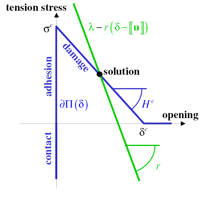
Figure 3.3-a : Behavior integration solution.
For the integration to be robust, it is necessary for the function between square brackets in to be strictly convex with respect to \(\delta\) (i.e. that the minimum is unique). By introducing \({H}_{c}\), the softening module of the cohesive law, we show a condition sufficient to satisfy this condition (see 5 for more details):
\(r>\underset{x\ge 0}{\text{max}}\mid {\psi }^{\text{'}\text{'}}(x)\mid =\frac{{\sigma }^{c}}{{\delta }^{c}}={H}^{c}\)
**Note:*
\(r=\text{100}\times {H}^{c}\) is a recommended value for the Code_Aster user.
It is now assumed that the condition is met, in addition the function in square brackets in is semi-continuous at the bottom, which guarantees the existence and uniqueness of the minimum.
Let’s now detail the numerical integration of the law, that is, the resolution of according to \(\tau =\lambda +r\left[\left[u\right]\right]\). Given the existence and uniqueness of the solution, it is interesting to use differential inclusion and the writing of the subdifferential provided by at. We thus find the four scenarios:
\(\text{si}\kappa =0\text{et}{\parallel \tau \parallel }_{+}\le {\sigma }^{c}={\psi }^{\text{'}}(0)\): perfect grip
\(\delta =0\)
\(\text{si}\kappa >0\text{et}{\parallel \tau \parallel }_{+}<\mathrm{r\kappa }\): return to zero with zero constraint
\(\delta =\frac{{\langle \tau \rangle }_{+}}{r}\)
\(\text{si}\kappa >0\text{et}\mathrm{r\kappa }\le {\parallel \tau \parallel }_{+}\le \mathrm{r\kappa }+{\psi }^{\text{'}}(\kappa )\): vertical discharge
\(\delta =\kappa \frac{{\langle \tau \rangle }_{+}}{{\parallel \tau \parallel }_{+}}\)
\(\text{si}\mathrm{r\kappa }+{\psi }^{\text{'}}(\kappa )<{\parallel \tau \parallel }_{+}\): damage
\(\delta ={\delta }_{\text{eq}}\frac{{\langle \tau \rangle }_{+}}{{\parallel \tau \parallel }_{+}};{\delta }_{\text{eq}}\text{solution de}{\psi }^{\text{'}}({\delta }_{\text{eq}})+{\mathrm{r\delta }}_{\text{eq}}={\parallel \tau \parallel }_{+}\)
**Note:*
the distinction \(\kappa =0\) or not is not necessary because appears as a special case of.
To conclude, the various regimes of cohesive law correspond to the \(\delta\) solutions provided by -. These are provided based on \(\tau =\lambda +r\left[\left[u\right]\right]\). No numerical method is necessary, in fact, the only equation to be solved (in) is piecewise linear.