2. Construction of the mixed interface finite element#
2.1. Principle of energy minimization in fracture mechanics#
In their approach to fracture mechanics, Frankfurt and Marigo 5 describe the state of a \(O\) structure by a field of displacement \(u\) that can admit discontinuities \(\delta =\left[\left[u\right]\right]\) across surfaces \(\Gamma (u)\). For a given loading, the displacement is characterized by an optimality condition: it corresponds to the local minimum of potential energy defined as the sum of the elastic deformation energy, cohesive energy and the work of external forces:
\(\begin{array}{}{E}_{\text{pot}}(u)={E}_{\text{el}}(u)+{E}_{\text{fr}}(\left[\left[u\right]\right])-{W}_{\text{ext}}(u)\\ {E}_{\text{el}}(u)=\underset{\Omega /\Gamma (u)}{\int }\Phi (\epsilon (u))d\Omega ;{E}_{\text{fr}}(\delta )=\underset{\Gamma (u)}{\int }\Pi (\delta )\text{dS}\end{array}\)
where \(\epsilon\) refers to the deformation tensor, \(\Phi\) the deformation energy density (volume) and \(\Pi\) the cohesive energy density (surface). In this formulation, the mechanisms of rupture are considered to be reversible. Irreversibility will be introduced in the next part, using internal variables. The characteristics of the problem are deduced from minimization, namely:
the prediction of the crack path, since all possible discontinuous movements are taken into account;
a stress criterion for the initiation of the crack (see 5).
the cohesive law relates the discontinuity of displacement \(\delta\) to the traction vector \(t\) based on the (generalized) derivative of \(\Pi\);
contact conditions are managed via cohesive energy to which is added an indicator function preventing the interpenetration of the lips.
However, taking into account all possible discontinuous movements leads to numerical difficulties related to the discretization of functional space \(\text{BD}(O)\). In particular, allowing discontinuities across each of the finite elements leads to a dependence of the results on the mesh. Alternative works are being carried out, based on the regularization of 5 discontinuities or on the adaptation of the 5 mesh. However, the latter are limited to Griffith surface energies (without cohesive forces) and lead to significant numerical difficulties. This is why we are introducing a simplification into our model by considering that the surfaces potential displacement discontinuities \(\Gamma\) are postulated a priori and that they no longer depend on \(u\).
2.2. Search for a saddle point by a decomposition method — coordination#
Despite the postulate on the direction of cracking, energy minimization is not obvious given the non-derivability of surface energy. We are based here on the decomposition — coordination technique introduced in 5, which condenses non-differentiability at a local level (Gauss points).
2.2.1. Augmented Lagrangian#
The relationship between the discontinuity field \(\delta\) and the displacement field \(u\) is explicitly introduced into the minimization, the total energy E therefore depends explicitly on \(u\) and on \(\delta\):
\(E(u,\delta )=\underset{\Omega \setminus \Gamma }{\int }\Phi (\epsilon (u))d\Omega -{W}_{\mathrm{ext}}(u)+\underset{\Gamma }{\int }\Pi (\delta )\mathrm{d\Gamma }\)
The minimization of the potential energy is then equivalent to the following minimization problem under stress (the displacement belonging to the set of kinematically admissible displacements):
\(\underset{\begin{array}{}u,\delta \\ \left[\left[u\right]\right]=\delta \end{array}}{\text{min}}E(u,\delta )\)
The linear constraint \(\left[\left[u\right]\right]=\delta\) is treated by dualization: a solution \((u,\delta )\) of corresponds to a saddle point \((u,\delta ,\lambda )\) of the following Lagrangian, where \(\lambda\) corresponds to the field of Lagrange multipliers:
\(L(u,\delta ,\lambda )\underset{\mathrm{déf}}{=}E(u,\delta )+\underset{\Gamma }{\int }\lambda \cdot (\left[\left[u\right]\right]-\delta )\mathrm{d\Gamma }\)
Finally, in order to gain greater coercivity compared to \(\delta\), which will later prove to be necessary, a quadratic penalization term is added that has no influence on the solution since it is equal to zero when the constraint is verified. The increased Lagrangian \({L}_{r}\), with the penalty coefficient \(r\), is then written:
\({L}_{r}(u,\delta ,\lambda )\underset{\mathrm{déf.}}{=}E(u,\delta )+\underset{\Gamma }{\int }\lambda \cdot (\left[\left[u\right]\right]-\delta )\mathrm{d\Gamma }+\underset{\Gamma }{\int }\frac{r}{2}{(\left[\left[u\right]\right]-\delta )}^{2}\mathrm{d\Gamma }\)
2.2.2. Characterization of the saddle point#
The first-order optimality conditions for augmented Lagrangian are written as follows:
\(\forall \mathrm{\delta \delta }\underset{\Gamma }{\int }\left[t-\lambda -r(\left[\left[u\right]\right]-\delta )\right]\cdot \mathrm{\delta \delta }=0\text{avec}t\in \partial \Pi (\delta )\)
\(\forall \mathrm{\delta u}\underset{\Omega \setminus \Gamma }{\int }\sigma :\epsilon (\mathrm{\delta u})+\underset{\Gamma }{\int }\left[\lambda +r(\left[\left[u\right]\right]-\delta )\right]\cdot \left[\left[\mathrm{\delta u}\right]\right]={W}_{\text{ext}}(\mathrm{\delta u})\text{avec}\sigma =\frac{\partial \Phi }{\partial \epsilon }(\epsilon )\)
\(\forall \mathrm{\delta \lambda }\underset{\Gamma }{\int }(\left[\left[u\right]\right]-\delta )\cdot \mathrm{\delta \lambda }=0\)
The meaning of subdifferential \(\partial \Pi\) is given in part 3. At this point, we’re just saying that \(t\in \partial \Pi (\delta )\) means that \(t\) and \(\delta\) are connected by the cohesive law. The equation therefore gives an interpretation of the Lagrange multiplier \(\lambda\): apart from the term penalization, these are cohesive forces. The equation expresses the balance of forces in the volume and along the surface of the discontinuity \(\Gamma\). Finally, imposes the constraint between the field of movement and its discontinuities.
2.3. Discretization of the finite element#
Since the trajectory of crack \(\Gamma\) is defined a priori and thanks to the hypothesis of small disturbances, the spatial discretization of the system - can be based on a finite interface element. Assume that subdomains \({O}_{-}\) and \({O}_{+}\) (parts of \(O\) below and above \(\Gamma\) respectively) are discretized by tetrahedra or hexahedra so that the nodes on either side of \(\Gamma\) coincide [1] _ . In this case, degenerate prisms or hexahedra can be used to discretize \(\Gamma\) and connect the two lips \({\Gamma }_{-}\) and \({\Gamma }_{+}\) of the potential cohesive crack (see Figure 2.3-a).
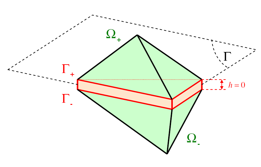
Figure 2.3-a : Discretization by finite interface element.
Let’s say a mesh characterized by the parameter \(h\) (for example, the maximum size of finite elements). In domain \(O\) we adopt a quadratic interpolation with classical Lagrange finite elements (P2-continuous). The discretized space of travel fields \({U}_{h}\) is written as:
\({U}_{h}=\left\{u;\forall x\in \Omega u(x)=\left[N(x)\right]\left\{U\right\}\right\}\)
where \(\left\{U\right\}\) designates the vector of nodal displacements and \(\left[N\right]\) the matrix of functions of quadratic forms. The displacement trace interpolated on \({\Gamma }_{-}\) and \({\Gamma }_{+}\) is also quadratic piecewise and the displacement discontinuity is expressed as follows:
\(\forall x\in \Gamma {u}_{\mid {\Gamma }_{-}}(x)=\left[{N}_{-}(x)\right]\left\{U\right\};{u}_{\mid {\Gamma }_{+}}(x)=\left[{N}_{+}(x)\right]\left\{U\right\}\)
\(\forall x\in \Gamma \left[\left[u(x)\right]\right]=\left[D(x)\right]\left\{U\right\}\text{avec}\left[D(x)\right]\underset{\text{déf.}}{=}\left[{N}_{+}(x)\right]-\left[{N}_{-}(x)\right]\)
where \(\left[{N}_{-}\right]\) and \(\left[{N}_{+}\right]\) correspond respectively to the trace of \(\left[N\right]\) on \({\Gamma }_{-}\) and \({\Gamma }_{+}\) and where \(\left[D\right]\) designates the matrix of functions of quadratic forms that interpolates the displacement jump. Note that it may be useful to introduce a rotation in \(\left[D\right]\) in order to obtain the components of \(\left[\left[u\right]\right]\) in a local coordinate system and thus distinguish the parts normal and tangential.
The Lagrange multiplier field \(\lambda\) is interpolated to \(\Gamma\) by piecewise linear form functions (P1—continuous), leading to the discretized space of the following Lagrange multipliers \({L}_{h}\):
\({L}_{h}=\left\{\lambda ;\forall x\in \Gamma \lambda (x)=\left[L(x)\right]\left\{\Lambda \right\}\right\}\)
where \(\left\{\Lambda \right\}\) corresponds to the nodal unknowns of the Lagrange multiplier and \(\left[L\right]\) refers to the matrix of functions of linear forms on \(\Gamma\). In this way, the constraint \(\left[\left[u\right]\right]=\delta\) imposed by is only realized in the weak sense.
Finally, the discretization of the discontinuity field \(\delta \in {D}_{h}\) is based on the collocation points on \(\Gamma\), with coordinates \({x}_{g}\). These points correspond to the Gauss points, of weight \({\omega }_{g}\), used to calculate integrals. A distinction is made here between standard modeling and so-called sub-integrated modeling.
In standard modeling, Gauss points are 3 (segments), 6 (triangles), or 9 (quadrilaterals) per element. This corresponds to a P2-discontinuous interpolation of \(\delta\). This choice has the advantage of limiting the risk of zero pivots appearing in the tangent matrix, but it does not satisfy condition LBB within the limit of an infinite \(r\) penalty parameter.
In sub-integrated modeling, there are 2 (segments), 3 (triangles), or 4 (quadrilaterals) Gauss points per element. This corresponds to a P1-discontinuous interpolation of \(\delta\). This choice better verifies condition LBB in the \(r\to \infty\) limit, but it is likely to cause zero pivots to appear in the tangent matrix. These zero pivots appear when the stiffness of the elements in contact with the interface is not sufficient to ensure the coercivity of the formulation, in particular when the interface is located on a plane of symmetry, or between a volume and a structural element (bar, grid or membrane).
Spatial discretization, notations, and finite element schemes for sub-integrated modeling are summarized on Figure 2.3-b.
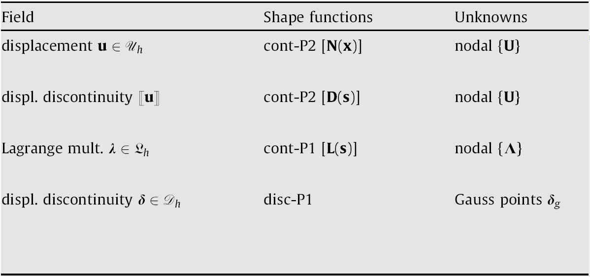
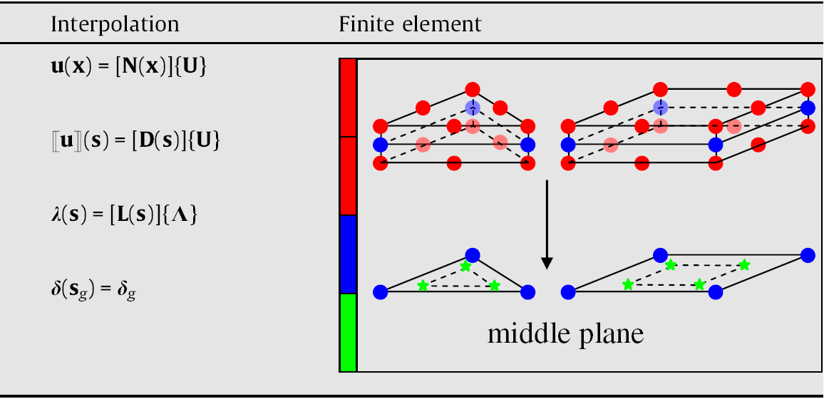
Figure 2.3-b : Spatial discretization
Field \(\delta\) disappears from the overall formulation thanks to static condensation. In fact, with the discretization adopted, the resolution is equivalent to satisfying the cohesive law at each collocation point:
\({t}_{g}={\lambda }_{g}+r(\left[\left[{u}_{g}\right]\right]-{\delta }_{g})\in \partial \Pi ({\delta }_{g})\text{avec}\{\begin{array}{cc}\left[\left[{u}_{g}\right]\right]=\left[{D}_{g}\right]\left\{U\right\}& ;\left[{D}_{g}\right]=\left[D({x}_{g})\right]\\ {\mu }_{g}=\left[{L}_{g}\right]\left\{\Lambda \right\}& ;\left[{L}_{g}\right]=\left[L({x}_{g})\right]\end{array}\)
The integration of the constitutive relationship (i.e. the resolution of, cf. next part), makes it possible to calculate \({\delta }_{g}\) as a function of \(\left\{U\right\}\) and \(\left\{\Lambda \right\}\), which is denoted by \(\delta\):
\({t}_{g}={\lambda }_{g}+r(\left[\left[{u}_{g}\right]\right]-{\delta }_{g})\in \partial \Pi ({\delta }_{g})\iff {\delta }_{g}=\stackrel{ˆ}{\delta }(\left[\left[{u}_{g}\right]\right],{\lambda }_{g})=\delta (U,\Lambda )\)
The \(r\) penalty parameter ensures the uniqueness of regardless of \(\left\{U\right\}\) and \(\left\{\Lambda \right\}\) (see next part). This is a necessary condition to ensure the robustness of the model.
We then have the nonlinear system whose unknowns are the nodal displacements \(\left\{U\right\}\) and the nodal Lagrange multipliers \(\left\{\Lambda \right\}\):
\(\underset{\Omega \setminus \Gamma }{\int }{\left[\nabla N\right]}^{T}\text{:σ}(U)+\sum _{g}{\omega }_{g}{\left[{D}_{g}\right]}^{T}\cdot (\left[{L}_{g}\right]\left\{\Lambda \right\}+r\left[{D}_{g}\right]\left\{U\right\}-r\delta (U,\Lambda ))=\left\{{F}_{\text{ext}}\right\}\)
\(\sum _{g}{\omega }_{g}{\left[{L}_{g}\right]}^{T}\cdot (\left[{D}_{g}\right]\left\{U\right\}-\delta (U,\Lambda ))=0\)
The volume integral and the nodal vector of external forces are calculated in the usual way. Finally, the system is solved simultaneously with respect to \(\left\{U\right\}\) and \(\left\{\Lambda \right\}\) using a Newton method (generalized), where the tangent operator is symmetric since - corresponds to a search for a saddle point.