3. The 2D-beam connection#
3.1. Objective#
As for the 3D/beam connection, the objective is to be able to represent a part of a complex slender structure ([Figure 3.1-a]) by a beam whose part to be analyzed is relatively « far away ». The aim of schematization by a beam is to bring realistic boundary conditions to the edges of the modelled and meshed part in a 2D continuous medium. These boundary conditions can be brought about by a beam, but also by discrete elements. The 2D/beam connection must therefore meet the following requirements:
P1 |
To be able to transmit beam forces to the 2D mesh |
P2 |
Do not generate “parasitic” constraints (or even a concentration of constraints), because the connection should then be placed far enough away from the area to be analyzed so that these disturbances are attenuated in the study area. |
P3 |
Do not favor kinematic conditions or static connection conditions over each other. It must be equivalent to bringing a torsor of effort or displacement to the limits of the 2D domain. |
P4 |
Admit any behaviors on either side of the connection (elasticity, plasticity…) and also allow dynamic analysis. |
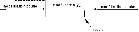
Figure 3.1-a
The process:
As for the 3D/beam connection, the 2D displacement field is broken down into a « beam » part and a « complementary » part. This leads us to define the kinematic connection conditions between the beam and the 2D structure as the equality of the beam displacement and the beam part of the 2D displacement field. Once this is done, the connection conditions are then interpreted in static terms and the static connection conditions are thus obtained.
The reader is invited to consult paragraph 2 (Le raccord 3D-poutre) which explicitly describes the method of the approach opposite. It will easily make the link with the 2D case.
3.2. Implementation of the connection method#
For each connection, the user must define:
S: |
The edge of the 2D surface: it is made by the keywords MAILLE_1et /or GROUP_MA_1; that is, it gives the list of linear meshes (\(\mathrm{lma}\)) (with 2D modeling “edge” elements) that geometrically represent this section. |
P: |
a node (keyword NOEUD_1ou GROUP_NO_1) carrying the 3 classical beam degrees of freedom: \(\mathrm{DX}\), \(\mathrm{DY}\), \(\mathrm{DRZ}\) |
Note:
**the node* \(P\) can be a beam element node or a discrete element node,
the list of meshes \(\mathrm{lma}\) must represent the section of the beam.
For each node, the program calculates the coefficients of the 3 linear relationships [éq 2.3-8] that link:
the 3 degrees of freedom of node \(P\),
with the degrees of freedom of**all* the nodes of \(\mathrm{lma}\).
These linear relationships will be dualized, like all linear relationships derived for example from the LIAISON_DDL keyword in AFFE_CHAR_MECA.
The calculation of the coefficients of linear relationships is carried out in several steps:
calculation of elementary quantities on the elements of \(\mathrm{lma}\): (OPTION: CARA_SECT_POUT3)
\({\mathrm{\int }}_{\text{elt}}1;{\mathrm{\int }}_{\text{elt}}x;{\mathrm{\int }}_{\text{elt}}y;{\mathrm{\int }}_{\text{elt}}{x}^{2};{\mathrm{\int }}_{\text{elt}}{y}^{2}\)
summation of these quantities on edge \((S)\), hence the calculation of:
\(A=\mid S\mid\)
\(G\) position
inertia tensor \(\Omega\)
knowing \(G\), elementary calculation on the elements of \(\mathrm{lma}\) of: (OPTION: CARA_SECT_POUT4)
\({\int }_{\text{elt}}\text{Ni};{\int }_{\text{elt}}\text{xNi};{\int }_{\text{elt}}\text{yNi};\text{où :}\begin{array}{c}\text{GM}=\left\{x,y\right\}\\ \text{Ni}=\text{fonctions de forme de l'élément}\end{array}\)
« assembly » of the terms calculated above to obtain, for each of the nodes of \(\mathrm{lma}\), the coefficients of the terms of the linear relationships.