5. Procedure: the routines to write#
It is at this level that the choice of the type of integration must be made. There are four options:
Use the architecture of the explicit integration environment with a Runge-Kutta schema of order 2 [R5.03.14] (ALGO_INTE =” RUNGE_KUTA “) :
this is the easiest method. In addition to retrieving material data, all you have to do is write a routine that calculates the derivatives of the internal variables.
the calculation of the tangent operator is not available in this environment, it is the elastic stiffness operator that is used
« Complete » implementation of the new behavior in the implicit integration environment PLASTI [R5.03.14] ( ALGO_INTE =” NEWTON “) :
resolution of the local nonlinear system by Newton’s method. In addition to recovering material data, it is necessary to write several routines called in the local Newton algorithm (evaluation of the threshold, calculation of the residue, analytical calculation of the Jacobian matrix…)
The coherent operator is obtained directly from the Jacobian of the local system, and the tangent operator in prediction is by default the elastic stiffness operator
PLASTI does not allow you to obtain compute-time optimized models
« Easy » implementation of the new behavior in the implicit integration environment PLASTI with [R5.03.14] ( ALGO_INTE =” NEWTON_PERT “) :
the local non-linear system can be rewritten so that the evaluation of the residue requires the developer only to specify the expression of the derivatives of the internal variables written in the framework of method 2 (explicit integration by RK2). We can therefore also perform an implicit integration in PLASTI with the only two routines necessary for the explicit integration.
The Jacobian of the local system is calculated by disturbance, so the calculation is even more expensive than with method 2. In the same way, the coherent tangent operator is obtained directly from the Jacobian of the local system
Create an autonomous routine for the complete integration of behavior:
often makes it possible to obtain the most efficient models (for example, by reducing the system to be solved to a single scalar, non-linear equation, see for example [R5.03.04], [R5.03.16], [], [R5.03.21],…)
requires more work « on paper » to optimize the equations
Attention :
In case 4, we will choose a routine number nn*and write the routine* lc00nn. In other cases we will choose the number 32 as an entry point: LC0032 call PLASTI or NMVPRK (Runge-Kutta) depending on the value of ALGO_INTE chosen by the user.
5.1. First possibility: introduce a new explicit behavior — diagram of RUNGE - KUTTA#
This type of integration corresponds to ALGO_INTE =” RUNGE_KUTTA “, which is the fastest way to introduce new behavior.
First, a routine XXXMATappelée must be written by the routing routine LCMATEafin to retrieve the material parameters and the size of the non-linear differential system to be integrated.
MATCST, NDT, NDI, NR, NVI, VIND)
Input arguments:
IMAT: material address MOD: modeling type NMAT: dimension of MATERD/MATERF
Output arguments:
MATERF: material coefficients a t+dt MATERx (,1) = elastic characteristics MATERx (,2) = plastic characteristics MATCST: “yes” if material a t = material a t+dt “no” otherwise NDT: total number of tensor components NDI: number of direct tensor components NR: number of components of the nonlinear system NVI: number of internal variables
Below is an example for each of the two main functions that this routine should perform.
AFFECTATION DES DIMENSIONS FROM PROBLEME LOCAL (NDT, NDI, NR, NVI)
IF (MOD .EQ.”3D”) THEN NDT = 6 NDI = 3 NR = NDT +2 ELSE IF (MOD .EQ. “D_ PLAN “.OR. MOD .EQ. “AXIS”) THEN NDT = 4 NDI = 3 NR = NDT +2 ELSE CALL U2 MESS (“F”,…) ENDIF
RECUPERATION OF MATERIAU
NOMC (2) = “NAKED” NOMC (3) = “ALPHA” NOMC (4) = “SY” NOMC (5) = “D_ SIGM_EPSI “ CALL RCVALB (FAMI, KPG, KSP, “-”, “-”, IMAT, “”, “”, “ELAS “,0,” “, & 0.D0.3, NOMC (1), MATERD (1.1), (1), (1.1), ICODRE (1) CALL RCVALB (FAMI, KPG, KSP, “-”, “-”, IMAT, “”, “”, “ECRO_LINE “,0,” “, & 0.D0.2, NOMC (4), MATERD (1.2), (4), (1.2), ICODRE (1)
You must then write a routine RKDXXX called by the routing routine LCDVIN and giving the time derivatives of the internal variables.
Routine examples RKDXXX: RKDCHA, RKDVEC, RKDHAY.
5.2. Second possibility: « complete » introduction of new behavior in PLASTI (implicit)#
This type of integration corresponds to ALGO_INTE =” NEWTON “. The PLASTI environment makes it possible to systematically integrate non-linear behavioral relationships using a local Newton method (at the level of the Gauss point). Knowing the constraints and the internal variables at time \(i-1\) as well as the total deformation increment \(\Delta {\epsilon }_{i}^{n}\) given by the global Newton algorithm, the local system of equations to be solved in purely implicit form is written as follows:
\(R(\Delta y)\mathrm{=}(\begin{array}{c}g(\Delta y)\\ l(\Delta y)\\ f(\Delta y)\end{array})\mathrm{=}0\) with \(\Delta y\mathrm{=}(\begin{array}{c}\Delta \sigma \\ \Delta \text{vari}\\ \Delta p\end{array})\)
The first equation represents for example the elastic stress-strain relationship (6 equations with 6 unknowns), with \(\mathrm{A}\) the elasticity operator (possibly modified for laws with damage), \(\Delta {\varepsilon }^{p}\) the variation in plastic deformation and \(\Delta {\varepsilon }^{\mathit{th}}\) the variation in thermal deformation:
\(g(\Delta y)\mathrm{=}\Delta \sigma \mathrm{-}\mathrm{A}(\Delta {\varepsilon }_{i}^{n}\mathrm{-}\Delta {\varepsilon }^{\mathit{th}}\mathrm{-}\Delta {\varepsilon }^{p})\mathrm{=}0\)
the second represents all the laws of evolution of the various scalar and/or vector internal variables (\({n}_{v}\) scalar equations with \({n}_{v}\) unknown)
\(l(\Delta y)\mathrm{=}0\)
the last represents the possible plasticity criterion (1 equation)
\(f(\Delta y)\mathrm{=}0\)
This system of \(6+{n}_{v}(+1)\) equations with \(6+{n}_{v}(+1)\) unknowns is solved by a Newton method:
\(\mathrm{\{}\begin{array}{c}\frac{\mathrm{\partial }R}{\mathrm{\partial }\Delta y}(\Delta {y}_{k})\mathrm{.}d\mathrm{[}\Delta {y}_{k}\mathrm{]}\mathrm{=}\mathrm{-}R(\Delta {y}_{k})\\ \Delta {y}_{k+1}\mathrm{=}\Delta {y}_{k}+d(\Delta {y}_{k})\end{array}\)
At convergence, we therefore obtain the increments of constraints and internal variables. For its part, the coherent tangent operator is calculated systematically from the Jacobian of the local system by routine LCOPTG (see [R5.03.14] for the details of the equations). It is therefore necessary to program at least one routine defining the residue (formed from the equations above) as well as a routine constructing the Jacobian matrix. The general architecture of PLASTI is briefly described below, with a list of routines to be written as you go.
General architecture of PLASTI :
→ writing a specific routine XXXMAT for retrieving material identical to RUNGE_KUTTA
IF (OPT .EQ. “RAPH_MECA” .OR. OPT .EQ. “FULL_MECA”) THEN INTEGRATION ELASTIQUE SUR DT CALL LCELAS (…) → possible writing of a specific routine XXXELA (by default) LCELIN: elasticity (linear)
PREDICTION ETAT ELASTIQUE A T+DT CALL LCCNVX (… , SEUIL) → writing a specific routine XXXCVX for evaluating the threshold
IF (SEUIL .GE. 0.D0) THEN CALL LCPLAS (…) ENDIF ENDIF
Routine LCPLAS calls LCPLNL, which performs the Newton loop whose structure is as follows:
Ratings:
YD= (SIGD, VIND): vector of the unknowns (of dimension \(6+{n}_{v}\)) at time T
YF= (SIGF, VINF): vector of the unknowns at the time T+DT
DY: increment of the vector of unknowns between the times Tet T+DT
DDY: vector increment of unknowns between two successive Newton iterations
R: residue
DRDY: Jacobian
So we solve: R (DY) = 0
By a Newton method DRDY (DYK) DDYK = - R (DYK)
DYK +1 = DYK + DDYK (DY0 DEBUT)
and we update YF = YD + DY
CALCUL OF THE SOLUTION D ESSAI INITIALE OF THE SYSTEME NL EN DY
CALL LCINIT (… DY,…) → possible writing of a specific routine XXXINI (by default DY is initialized to 0)
ITERATIONS OF NEWTON
ITER = 0 1 CONTINUE ITER = ITER + 1
INCREMENTATION BY YF = YD + DY
CALL LCSOVN (NR, YD, DY, YF)
CALCUL DES TERMES FROM SYSTEME TO T+DT = -R (DY)
CALL LCRESI (… , DY, R, IRET) → writing a specific routine XXXRES for calculating the residue
CALCUL FROM JACOBIEN FROM SYSTEME TO T+DT = DRDY (DY)
If ALGO_INTE =” NEWTON “exact calculation of the Jacobian CALL LCJACB (… DY,… DRDY, IRET) → writing a specific routine is required XXXJAC 5.3 otherwise if ALGO_INTE =” NEWTON_PERT “, calculation by disturbance (cf §) CALL LCJACP (… DRDY,…)
RESOLUTION FROM SYSTEME LINEAIRE DRDY (DY). DDY = -R (DY)
CALL LCEQMN (NR, DRDY, DRDY1) CALL LCEQVN (NR, R, DDY) CALL MGAUSS (“NCWP”, DRDY1, DDY, NR, NR,1, RBID, IRET)
REACTUALISATION BY DY = DY + DDY
CALL LCSOVN (NR, DDY, DY, DY)
RECHERCHE LINEAIRE in the case ALGO_INTE =” NEWTON_RELI “
CALL LCRELI (…)
ESTIMATION FROM CONVERGENCE
CALL LCCONV (DY, DDY, NR, ITMAX, TOLER,… , R,… , IRTET) → possible writing of a specific routine XXXCVG of the criterion of convergence (relative criterion by default in LCCONG) IF (IRTET .GT.0) GOTO 1
CONVERGENCE -> INCREMENTATION FROM YF = YD + DY
CALL LCSOVN (NDT + NVI, YD, DY, YF)
MISE TO JOUR OF SIGF, VINF
CALL LCEQVN (NDT, YF (1), SIGF) CALL LCEQVN (NVI -1, YF (NDT +1), VINF)
In summary, for a « complete » introduction of a new behavior in PLASTI, you must write the following specific routines:
XXXMAT called by LCMATE: recovery of the material and the size of the local problem
XXXCVX called by LCCNVX: threshold assessment
XXXRES called by LCRESI: calculation of the residue
XXXJAC called by LCJACB: Jacobian calculation
It may also be useful, as needed, to write the following specific routines:
XXXELA called by LCELAS: elastic integration (if non-linear elasticity)
XXXINI called by LCINIT: initialization (for initialization other than DY0 =0)
XXXCVG called by LCCONV: to modify the convergence criterion
5.3. Third possibility: use of explicit integration routines in an implicit integration with PLASTI#
5.3.1. Principle#
This last case corresponds to ALGO_INTE_ =” NEWTON_PERT “* , it is the « easy » method of implementing the new behavior in the implicit integration environment PLASTI. It is possible to directly use the two routines XXXMAT and RKDXXX (retrieving material data, and derivatives of internal variables) used with ALGO_INTE_ =” RUNGE_KUTTA “to perform an implicit integration. In fact, the system of differential equations solved by RUNGE_KUTTA can be written as:
\(\mathrm{\{}\begin{array}{c}\Delta \sigma \mathrm{=}\mathrm{A}(\Delta {\varepsilon }_{i}^{n}\mathrm{-}\Delta {\varepsilon }^{\mathit{th}}\mathrm{-}\Delta {\varepsilon }^{p}(Y))\\ \frac{dY}{dt}\mathrm{=}F(Y,t;\sigma )\end{array}\)
where \(Y\) represents all the internal variables of the model. The relationship between the stress tensor and the elastic part of the strain tensor is generally linear, but can be evaluated nonlinearly by a specific expression.
Once the routine RKDXXX to calculate \(\frac{dY}{dt}\mathrm{=}F(Y,t;\sigma )\) has been programmed, it is possible to use it for an implicit integration, which consists in solving (cf. [R5.03.14]):
\(R(\Delta Z)\mathrm{=}0\mathrm{=}\left[\begin{array}{c}{R}_{1}(\Delta Z)\\ {R}_{2}(\Delta Z)\end{array}\right]\), with \(\Delta Z\mathrm{=}(\begin{array}{c}\Delta \sigma \\ \Delta Y\end{array})\mathrm{=}Z(t+\Delta t)\mathrm{-}Z(t)\)
The first system of equations represents the relationship between stress and elastic deformation
\({R}_{1}(\Delta Z)\mathrm{=}{A}^{\mathrm{-}1}\sigma \mathrm{-}(\Delta {\varepsilon }_{i}^{n}\mathrm{-}\Delta {\varepsilon }^{\mathit{th}}\mathrm{-}\Delta {\varepsilon }^{p}(Y))\mathrm{=}{A}^{\mathrm{-}1}\sigma \mathrm{-}G(Y)\mathrm{=}0\)
By convention, the first values of \(Y\) represent the variation in plastic deformation, to facilitate the calculation of \(G(Y)\) (see routine LCRESA for more details)
The second expresses the laws of evolution of the various internal variables, i.e. after time discretization by an implicit Euler schema:
\({R}_{2}(\Delta Z)\mathrm{=}\Delta Y\mathrm{-}\Delta t\mathrm{.}F(Y,\sigma )\mathrm{=}0\)
This system is solved by the Newton method proposed in environment PLASTI and described in the previous paragraph:
\(\mathrm{\{}\begin{array}{c}\frac{\mathrm{\partial }R}{\mathrm{\partial }\Delta Z}d(\Delta {Z}_{k})\text{= -}R(\Delta {Z}_{k})\\ \Delta {Z}_{k\text{+}1}\text{=}\Delta {Z}_{k}\text{+}d(\Delta {Z}_{k})\end{array}\)
The quantities \(G\) and \(F\) occurring in the residue are calculated by the « explicit » routine RKDXXX to be written, and the residue is automatically constructed by the routine LCRESA. The Jacobian matrix is automatically calculated by disturbance (routine LCJACP). For its part, the coherent tangent operator is calculated systematically using the Jacobian method (routine LCOPTG, see [R5.03.14] for the details of the equations).
In summary, this method makes it possible, with the only two routines necessary for explicit integration, (material coefficients and calculation of the derivatives of the internal variables) to use an implicit integration, and to benefit from a tangent matrix. This process is economical in terms of development time, but a priori less efficient in time CPU than an explicitly programmed Jacobian matrix.
The calculation of the tangent operator by disturbance is detailed below, as well as the convergence criterion of the local Newton algorithm.
Perturbation calculation (LCJACP) : finite differences of order 2
Initialization of the disturbance: \(\eta \mathrm{=}{10}^{\mathrm{-}7}∣∣\Delta Z∣∣\)
loop over columns \(j\) of the matrix to be filled in:
calculation of \(R(\Delta Z+\eta {I}_{j})\) with \({I}_{j}={[00\dots 1\dots 00]}^{T}\) zero vector except on line \(j\)
calculation of \(R(\Delta Z\mathrm{-}\eta {I}_{j})\)
calculation of column \(j\): \({\left[\frac{\mathrm{\partial }R}{\mathrm{\partial }\Delta Z}\right]}_{\text{...},j}\mathrm{\simeq }\frac{R(\Delta Z+\eta {I}_{j})\mathrm{-}R(\Delta Z\mathrm{-}\eta {I}_{j})}{2\eta }\)
Convergence criterion (LCCONG) :
The two blocks \({R}_{1}\) and \({R}_{2}\) from the residue are separated to avoid problems due to different orders of magnitude. At each iteration \(k\) of the local Newton algorithm, we calculate:
\({\mathit{err}}_{1}\mathrm{=}\frac{{∣∣{R}_{1}(\Delta {Z}_{k})∣∣}_{\mathrm{\infty }}}{{∣∣{R}_{1}(\Delta {Z}_{0})∣∣}_{\mathrm{\infty }}}\), with \({R}_{1}(\Delta {Z}_{0})\mathrm{=}\Delta {\varepsilon }_{i}^{n}\) because we have \(\Delta {Z}_{0}\mathrm{=}0\) at initialization. (see § 5.2)
\({\mathit{err}}_{2}\mathrm{=}\frac{{∣∣{R}_{2}(\Delta {Z}_{k})∣∣}_{\mathrm{\infty }}}{{∣∣Y(t)+\Delta {Y}_{k}∣∣}_{\mathrm{\infty }}}\)
The stopping criterion is then as follows:
\(\mathit{max}({\mathit{err}}_{\mathrm{1,}}{\mathit{err}}_{2})<\xi\), where \(\xi\) is given by RESI_INTE_RELA.
5.3.2. example#
An example: Hayhurst’s visco-elasto-plastic law.
Routine for reading material coefficients (called by the routing routine LCMATT):
HAYMAT
Routine for calculating derivatives of internal variables (called by the routing routine LCDVIN):
RKDHAY
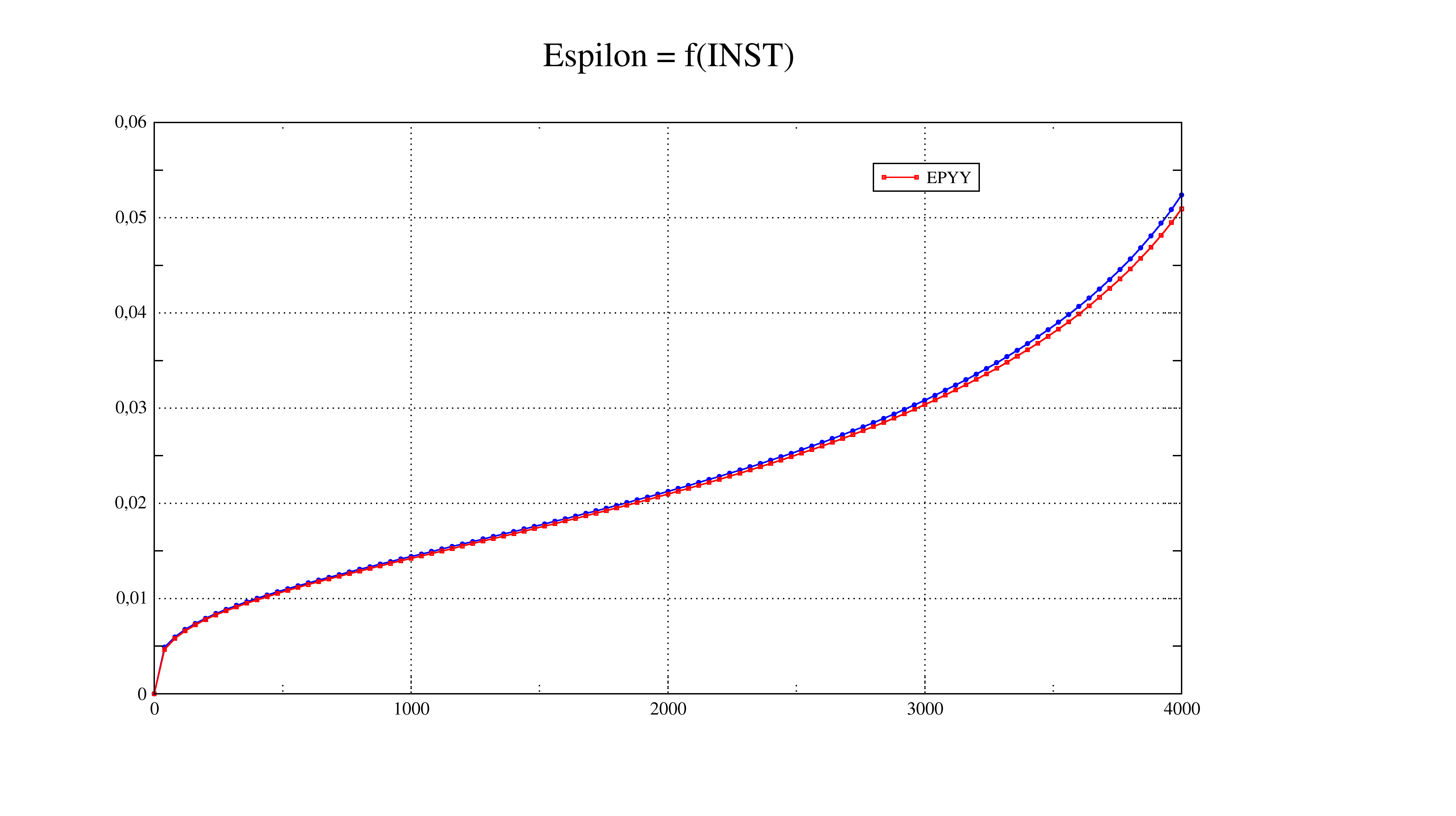
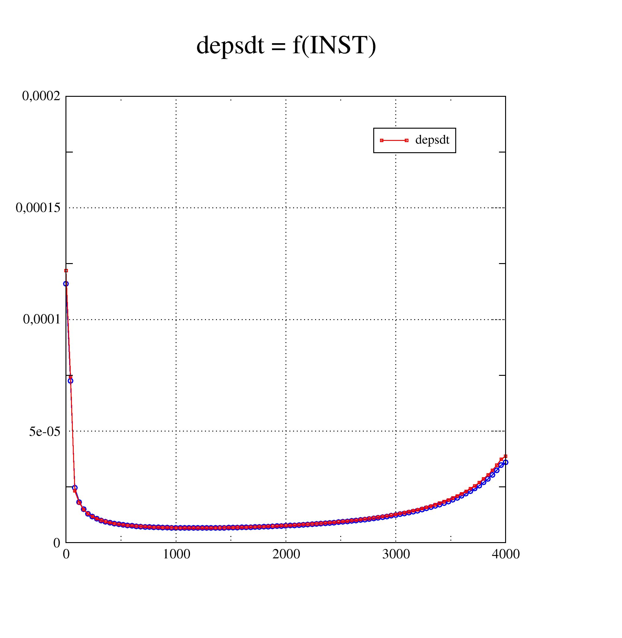
The explicit/implicit developments of this behavioral relationship are tested and compared in the ssnv225 test case [V6.04.225]. This is a hardware test of creep in large deformations to validate the capabilities of the HAYHURST model to represent primary, secondary and tertiary creep. Here are the execution characteristics for this test in version 11.2:
Modeling A: ALGO_INTE =” RUNGE_KUTTA “
time CPU: 90.59 s
Number of time steps: 1660
Number of Newton iterations: 7615
B modeling: ALGO_INTE =” NEWTON_PERT “:
time CPU: 27.38s
Number of time steps: 520
Number of Newton iterations: 1404
The results are almost identical:
5.4. Fourth possibility: write a standalone lc00nn routine#
lc00nn: routine relating to an element integration point, specific to a law of behavior ~~~~~~~~~~~~~~~~~~~~~~~~~~~~~~~~~~~~~~~~~~~~~~~~~~~~~~~~~~~~~~~~~~~~~~~~~~~~~~~~~~~~~~~~~~~~~~~~~~~~~~~~~~~~~~~~~~~~~~~~~~~~~~~~~~~~~~~~~~~~~~~~~~~~~~~~~~~~~~~~~~~~~~~~~~~~~~~~~~~~~~~~~~~~~~~ ~~~~~~
Search the bibfor/algorith directory for an unused routine number lc00nn (\((50<\mathit{nn}<100)\)) and start with this empty routine.
Note :
The call to lc00nn*by* lc0000 (which is the routine calling all the behavior integration routines available in co*de_* a*ster) is already written. However, you must ensure that the arguments (as well as the order of these arguments) chosen when declaring of* lc00nn*by the developer are the same as when calling in* lc0000*.*
The input arguments to an lc00nn routine are*a minima*:
FAMI gauss point family (RIGI, MASS,…)
KPG, KSP Gauss point and subpoint number
NDIM space dimension (\(\mathrm{3d}\mathrm{=}3\), \(\mathrm{2d}\mathrm{=}2\), \(\mathrm{1d}\mathrm{=}1\))
IMATE material address
COMPOR behavior info
compor (1) = behavior relationship (vmis_cine_…)
compor (2) = number of internal variables
compor (3) = type of deformation (small, green…)
CRIT local criteria
Write (1) = maximum number of iterations at convergence (ITER_INTE_MAXI)
crit (3) = convergence tolerance value (RESI_INTE_RELA)
INSTAM instant t-
INSTAP instant t = t- + dt
EPSM total deformation a t- (or possibly the transformation gradient depending on the type of deformation: the arguments of the calling routine, lc0000, contain the dimension of EPSM, and DEPS),
DEPS total deformation increment (same remark)
SIGM constraint a t-
VIM internal variables a t-
OPTION calculation option
RIGI_MECA_TANG -> dsidep (t)
FULL_MECA -> dsidep (t+dt), sig (t+dt)
RAPH_MECA -> sig (t+dt)
ANGMAS the three angles (nautical or Euler) of the massive keyword
TYPMOD modeling type: 3D, AXIS, D_ PLAN, C_ PLAN,…
ICOMP counter for the local redistribution of the time step
NVI number of internal variables of behavior
depending on the calculation option, the output arguments are:
VIP internal variables at the current time (options RAPH_MECA and FULL_MECA)
SIGP term of order 0 in the linearization of the constraint (option RIGI_MECA_TANG) — cf. § 4
constraints at the current moment (options RAPH_MECA and FULL_MECA)
DSIDEP coherent or velocity tangent operator (option FULL_MECA or RIGI_MECA_TANG).
CODRET return code to indicate (if it is not zero) an integration problem
local, so to redistribute the time step
Remarks:
L*where appropriate, it is possible to also use*a derived type as input (variable BEHinteg*in*LC0000/LCnnnn) .*This type*contains additional arguments, for example a characteristic length in the case of non-local models… *
Likewise, it is possible to transfer additional arguments to the output of the LCnnnn/LC0000 routine via the BEHinteg variable.
Attention, in the case RIGI_MECA_TANG , tables relating to constraints and internal variables at the end of the time step are not allocated. It is therefore not necessary to use them to calculate the tangent prediction matrix.
5.4.1. Organization of the writing routine#
As in § 3.3, we take the example of the Von Mises law of linear kinematic work hardening VMIS_CINE_LINE (num_lc=3 in vmis_cine_line.py):
& INSTAP, EPSM, DEPS, SIGM, VIM,,, OPTION, ANGMAS, SIGP, VIP, & TAMPON, TYPMOD, ICOMP, NVI,, DSIDEP, CODRET)
This routine is in fact a referral routine for behaviors VMIS_CINE_LINE and VMIS_ECMI_ *. The integration of VMIS_CINE_LINE is carried out in the NMCINE routine, called by lc0003 and whose content is described here briefly.
Note that in this example, the law follows the deform_ldc = “OLD” mechanism, and that as such, thermal deformations are calculated and subtracted within the law (see § 4).
LECTURE DES CARACTERISTIQUES ELASTIQUES FROM MATERIAU (TEMPS T = +)
NOMRES (1) =”E” NOMRES (2) =”NUD” CALL RCVALB (FAMI, KPG, KSP, “+”, “+”, IMATE, “”, “”, “ELAS “,0,” “, & 0.D0.2, NOMRES, VALRES,, ICODRE, 2) E = VALRES (1) NUDE = VALRES (2)
Note:
RCVALB is a general routine for interpolating the values of the material coefficients in relation to the command variables on which they depend (see the utilities) .
RCVARCest a routine that allows you to retrieve the value of a control variable (temperature, drying, irradiation,…) at the moment in question, and at the Gauss point in question (see the utilities). Example:
CALL RCVARC (“”, “TEMP”, “-”, “-”, FAMI, KPG, KSP, TM, IRET)
CALL RCVARC (“”, “TEMP”, “”, “,” + “,” + “, FAMI, KPG, KSP, TP, IRET)
LECTURE DES CARACTERISTIQUES FROM ECROUISSAGE
NOMRES (2) =”SY” CALL RCVALB (FAMI, KPG, KSP, “+”, “+”, IMATE, “”, “”, “ECRO_LINE “,0,” “, & 0.D0.2, NOMRES, VALRES,,, ICODRE, 2) DSDE = VALRES (1) SIGY = VALRES (2) C = 2.D0/3.D0* DSDE/(1.D0- DSDE /E)
CALCUL DES CONTRAINTES ELASTIQUES AND SOME CRITERE FROM VON MISES
DO 110 K=1.3

DEPSTH (K) = DEPS (K) - EPSTHE

DEPSTH (K+3) = DEPS (K+3)

110 CONTINUE

EPSMO = (DEPSTH (1) + DEPSTH (2) + DEPSTH (3)) /3.D0

DO 115 K=1, NDIMSI

DEPSDV (K) = DEPSTH (K) - EPSMO * KRON (K)

115 CONTINUE

SIGMO = (SIGM (1) + SIGM (2) + SIGM (3)) /3.D0

SIELEQ = 0.D0

DO 114 K=1, NDIMSI

SIGDV (K) = SIGM (K) - SIGMO * KRON (K)

SIGDV (K) = DEUXMU/DEUMUM * SIGDV (K)

SIGEL (K) = SIGDV (K) + DEUXMU * DEPSDV (K)

SIELEQ = SIELEQ + (SIGEL (K) -C/CM*VIM (K))**2

114 CONTINUE

SIGMO = TROISK/TROIKM * SIGMO

SIELEQ = SQRT (1.5D0* SIELEQ)

SEUIL = SIELEQ — SIGY

DP = 0.D0

PLASTI = VIM (7)
CALCUL DES CONTRAINTES AND DES VARIABLES INTERNES
Expressions for constraints and internal variables (RAPH_MECA and FULL_MECA) are given in [R5.03.02]
IF (OPTION (1:9) .EQ. 'RAPH_MECA' .OR.

& OPTION (1:9) .EQ. 'FULL_MECA') THEN

IF (SEUIL .LT.0.D0) THEN

VIP (7) = 0.D0

DP = 0.D0

SIELEQ = 1.D0

A1 = 0.D0

A2 = 0.D0

ELSE

VIP (7) = 1.D0

DP = SEUIL/(1.5D0* (DEUXMU +C))

A1 = (DEUXMU/(DEUXMU +C)) * (SEUIL/SIELEQ)

A2 = (C/(DEUXMU +C)) * (SEUIL/SIELEQ)

ENDIF

PLASTI = VIP (7)

DO 160 K = 1, NDIMSI

SIGDV (K) = SIGEL (K) - A1*(SIGEL (K) - VIM (K)*C/CM)

SIGP (K) = SIGDV (K) + (SIGMO + TROISK *EPSMO)* KRON (K)

VIP (K) = VIM (K) *C/CM + A2* (SIGEL (K) - VIM (K) *C/CM)

160 CONTINUE

ENDIF
CALCUL FROM OPERATEUR TANGENT “DSIPSEP”: RIGI_MECA_TANG (in speed) or FULL_MECA (consistent)
IF (OPTION (1:14) .EQ. 'RIGI_MECA_TANG' .OR.

& OPTION (1:9) .EQ. 'FULL_MECA') THEN

CALL MATINI (6,6,0.D0, DSIDEP)

DO 120 K=1.6

DSIDEP (K, K) = DEUXMU

120 CONTINUE

IF (OPTION (1:14) .EQ. 'RIGI_MECA_TANG') THEN

DO 174 K = 1, NDIMSI

SIGDV (K) = SIGDV (K) - VIM (K) *C/CM

174 CONTINUE

ELSE

DO 175 K = 1, NDIMSI

SIGDV (K) = SIGDV (K) - VIP (K)

175 CONTINUE

ENDIF

SIGEPS = 0.D0

DO 170K = 1, NDIMSI

SIGEPS = SIGEPS + SIGDV (K) * DEPSDV (K)

170 CONTINUE

A1 = 1.D0/ (1.D0+1.5D0*(DEUXMU +C)*DP/ SIGY)

A2 = (1.D0+1.5D0*C*DP/ SIGY) *A1

IF (PLASTI .GE.0.5D0. AND. SIGEPS .GE.0.D0) THEN

COEF = -1.5D0*(DEUXMU/SIGY)**2/(DEUXMU +C) * A1

DO 135 K=1, NDIMSI

DO 135 L=1, NDIMSI

DSIDEP (K, L) = A2 *DSIDEP (K, L) + COEF* SIGDV (K) * SIGDV (L)

135 CONTINUE

LAMBDA = LAMBDA + DEUXMU **2*A1*DP/ SIGY /2.D0

ENDIF

DO 130 K=1.3

DO 131 L=1.3

DSIDEP (K, L) = DSIDEP (K, L) + LAMBDA

131 CONTINUE

130 CONTINUE

ENDIF
5.4.2. Control variables (external state variables)#
The dependence of the material parameters on the control variables (drying, temperature, etc.) is taken into account by using routine RCVALB. In addition, there are command variables specific to certain laws of behavior that must be calculated (generally at the element level) and not transmitted by the AFFE_MATERIAU/AFFE_VARC mechanism, these are:
ELTSIZE1: calculating the size of an element (for the BETON_DOUBLE_DP law);
ELTSIZE2: calculating the size of an element (for the ENDO_PORO_BETON law);
COORGA: coordinates of the element’s Gauss points (for the META_LEMA_ANI law);
GRADVELO: for the deformation rate gradient (for the MONOCRISTAL law);
HYGR: humidity (based on the desorption function FONC_DESORP).
Behavioral laws using these variables use the text_vari keyword in their catalog. The addition of another variable of this style requires specific development which cannot therefore be detailed here.
On the other hand, you can use the variables defined above. It is necessary to:
impact the catalog of the law of behavior and add this variable in exte_vari;
retrieve the value of this variable via the calculation module
Variables |
Variable (s) in the calculation module |
HYGR |
|
ELTSIZE1 |
|
ELTSIZE2 |
|
COORGA |
ca_vext_coorga_ (27.3) |
GRADVELO |
For example:
use calcul_module, only: ca_vext_gradvelo_
real (kind=8):: l (3,3)
integer:: i, j
Do i = 1, 3
Do j = 1, 3
l (i, j) =ca_vext_gradvelo_ (3* (i-1) +j)
End Do
End Do