3. Contents of the sd_fiss_xfem objects#

Preliminary remark on the distinction between 2D and 3D:

The presence of certain objects in the sd_fiss_xfem data structure sometimes depends on the dimension of the mesh on which the crack is represented. Thus, the distinction between 2D and 3D relates to the dimension of the mesh contained in the model given by the user under the MODELE keyword of the DEFI_FISS_XFEM command.

3.1. General objects#

3.1.1. . INFO#

The concept. INFO is a \(\mathit{K16}\) vector of length 3 containing general information.

The 1st component of this vector provides information on the type of discontinuity relating to the sd_fiss_xfem: either a crack or an interface. The 2nd component indicates the discontinuous field: either the displacement field or the constraint field. The 3rd component specifies whether the bottom is closed or open.

. INFO (1) = “FISSURE” or “INTERFACE”

. INFO (2) = “DEPL” or “SIGM”

. INFO (3) = “OUVERT” or “FERME”

The values of this vector are only accessed by the dismoi.f routine.

Example:

CALL DISMOI (“F”, “TYPE_DISCONTINUITE”, “”, FISS,, “FISS_XFEM”, IBID, TYPDIS, IRET)

CALL DISMOI (“F”, “CHAM_DISCONTINUITE”, “”, FISS,, “FISS_XFEM”, IBID, TYPCHA, IRET)

CALL DISMOI (“F”, “TYPE_FOND”, “”, FISS,, “FISS_XFEM”, IBID, TYPFON, IRET)

3.1.2. . MAILLAGE#

The concept. MAILLAGE is a K8 vector of length 1 containing the name of the mesh on which the crack is built (value of the MAILLAGE keyword as input to DEFI_FISS_XFEM). In case of propagation, this vector is duplicated from the old crack to the new crack.

This vector is accessed only by the dismoi.f routine.

Example:

CALL DISMOI (“F”, “NOM_MAILLAGE”, “”, FISS,, “FISS_XFEM”, IBID, MODELE, IRET)

3.2. Level set objects#

3.2.1. . CHAMPS. LVS#

The concept. CHAMPS. LVS is a boolean vector of length 1. If this vector is present (and its value is then always equal to TRUE), the level set fields for the current crack were given directly by the user (by DEFI_FISS_XFEM using the keywords CHAMP_NO_LSN and CHAMP_NO_LST) and they were not calculated.

If both fields were extracted from a crack propagated by PROPA_FISS, the domain location information (. PRO. RAYON_TORE (§ 3.4.1) and. PRO. NOEUD_TORE (§ 3.4.2)) and on the use of an auxiliary grid for the propagated crack (. GRI. MAILLAGE (§ 3.4.4),. GRI .L*NO (§ 3.4.5) and. GRI. GRL*NO (§ 3.4.6)) have been lost and the SD of the current crack does not contain them. In fact, this information is stored at the level of the SD fiss_xfem and not at the level of the SD field_no. This is a problem in the event that the current crack is propagated by PROPA_FISS because false results could be obtained. In fact, in cases where the location of the domain or the auxiliary grid were used, the level sets were updated only in a small domain around the bottom of the crack: in the first case this is obvious, and in the second case the level sets were projected onto the physical mesh with a projection domain localized regardless of the use of the location of a calculation domain at the bottom of the crack on the grid. Outside the location/projection domain, the value of the set levels is the same as that calculated to define the crack: the level sets are therefore not continuous at the limit of the location/projection domain and the description of the crack is therefore not correct throughout the mesh. If the information on the location domain and on the auxiliary grid is not stored in the SD of the new crack, PROPA_FISS propagates the crack assuming that the level sets are correct throughout the mesh. When the background of the propagated crack leaves the location/projection domain used for the initial crack before propagation, false results are obtained and there are convergence problems in the resetting and reorthogonalization of the level sets.

In the case where the level sets given to define the new crack were not extracted from a crack propagated by PROPA_FISS, or if the location of the domain or the auxiliary grid were not used with PROPA_FISS, the given level sets fields correctly represent the crack across the entire mesh and the propagation of the new crack can be calculated without problems by PROPA_FISS.

If this vector is present in the crack SD, PROPA_FISS emits an alarm for the user to check if it is not in the presence of a field extracted from a crack propagated with PROPA_FISS that he would use with the location of the calculation domain or with an auxiliary grid.

3.2.2. . LTNO and. LNNO#

The concept. LTNO (resp.. LNNO) is a scalar node field (CHAM_NO) that contains for each node of the mesh the real value of the level set tangent (resp. normal) to the crack.

3.2.3. . GRLTNO and. GRLNNO#

The concept. GRLTNO (resp.. GRLNNO) is a node field (CHAM_NO) with 3 real components. It contains for each node of the mesh the values of the tangent level set gradient (resp. normal) in the 3 directions of space.

Let \(i\) be the \(i\) th node of the mesh,

V =. GRLTNO (i);

V (1)	Value of the next \(x\) gradient of the tangent level set, calculated at the \(i\) th node
V (2)	Value of the next \(y\) gradient of the tangent level set, calculated at the \(i\) th node
V (3)	Value of the next \(z\) gradient of the tangent level set, calculated at the \(i\) th node

In 2D, we only have 2 components following \(x\) and \(y\).

3.2.4. . BASLOC#

The concept. BASLOC is a field with nodes (CHAM_NO) with 9 real components (in 3D). It contains the origin and the vectors of BASe LOCale at the bottom of the crack. For each node, the first three components are the coordinates of the node’s projected onto the background, which corresponds to the origin of the local base. The next three components are the coordinates of the 1st vector (GRLT) of the base. The last three components are the coordinates of the 2nd vector (GRLN) of the base. The 3rd vector in the base is not stored, because it is easily determined as being the vector product of the first 2 vectors.

Let \(i\) be the \(i\) th node of the mesh,

V =. BASLOC (i);

V (1)	Next coordinate \(x\) of the projected node i on the background
V (2)	Next coordinate \(y\) of the projected node i on the background
V (3)	Next coordinate \(z\) of the projected node i on the background
V (4)	Next coordinate \(x\) of the 1st vector of the local base
V (5)	Next coordinate \(y\) of the 1st vector of the local base
V (6)	Next coordinate \(z\) of the 1st vector of the local base
V (7)	Next coordinate \(x\) of the 2nd vector of the local base
V (8)	Next coordinate \(y\) of the 2nd vector of the local base
V (9)	Next coordinate \(z\) of the 2nd vector of the local base

In 2D, we only have 2 components following \(x\) and \(y\), i.e. 6 components for BASLOC. Recall that in 2D, either there is only one crack background, which is then a point (case of 2D through cracks) and in this case all the nodes of the mesh have the same projection on the crack background, or there are two crack bottoms, so two points (case of 2D cracks that do not open through) and in this case, some of the nodes of the mesh are projected onto the first crack background, so two points (case of 2D cracks that do not open through) and in this case, some of the nodes of the mesh are projected onto the first crack background and another part of the nodes of the mesh projects onto the 2nd crack bottom.

Notes:

For a discontinuous crack front, the projection used above must be carried out with care. A distinction should be made between two types of discontinuities:
- or the front is continuous but cut by a material discontinuity (hole in a piece) which generates a discontinuous front in the material, but extendable by continuity outside the material,
- or the front is really discontinuous in the definition of the crack to be propagated.

Before projection, it is first necessary to test whether the front is virtually continuous or if it is really discontinuous. To then detect the discontinuity of the crack front, we rely on a simple criterion which consists in testing the collinearity of the propagation vectors (1st vector of the local base) at the ends of the crack fronts between two consecutive fronts:

\(\mathit{acos}(\vec{{V}_{{P}_{\text{i}}}}\text{.}\vec{{V}_{{P}_{\text{i+1}}}})<10°\)

If the angular threshold above is exceeded (10° angle), the edge ending in \({P}_{\text{i}}\) and the edge beginning in \({P}_{\text{i+1}}\) are treated as two separate fronts when projecting each node onto the global crack front.

In two dimensions, it is convenient to « flip » the first vector of the local base (propagation vector) to change the sign of the plane shear mode (or mode 2) and obtain an always positive sign. This change is only done locally for post-processing purposes and does not impact the data structure described in this paragraph.

3.2.5. . FONDFISS#

The vector. FONDFISS is a real vector containing the coordinates of the points at the bottom of the crack. The points are ordered according to the method described in document [R7.02.12], so that a curvilinear abscissa can be defined.

If NFON is the number of points at the bottom of the crack, then the length of the vector. FONDFISS is 4x NFON. For each point at the bottom of the crack, the first 3 components correspond to the 3 coordinates (in 3D) of the point, and the fourth component is its curvilinear abscissa.

When the bottom is closed, the last point is equal to the first. The last 4 terms of the vector. FONDFISS are then identical to the first 4.

This structure is not modified in 2D. However, only the first 2 components are used, because neither the curvilinear abscissa nor the last geometric component are relevant in 2D.

This object is only created if there is at least one point at the bottom of the crack.

3.2.6. . BASEFOND#

The vector. BASEFOND is a real vector containing the local base associated with each point at the crack bottom.

If NFON is the number of points at the bottom of the crack and if NDIM is the dimension of the model (2 in 2D and 3 in 3D), then the length of the vector. BASEFOND is \(2\mathrm{\times }\mathit{NDIM}\mathrm{\times }\mathit{NFON}\). In fact, this vector contains, successively for all the bottom points, the components (2 in 2D and 3 in 3D) of the vector normal to the plane of the crack and of the direction of propagation (vector tangent to the plane of the crack).

In 3D, when the background is closed, the last point is equal to the first. The last 4 terms of the vector. BASEFOND are then identical to the first 4.

3.2.7. . FONDMULT#

In 3D, the crack bottom is a line that is either closed (non-opening crack) or open (through crack). In most cases, the crack bottom is a solid line, like the circular crack shown in Figure 3.2.7-1.

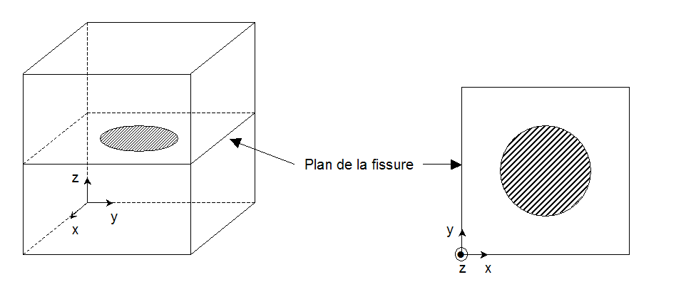
Figure 3.2.7-1 Case of a continuous crack background.

However, it may happen that the bottom of the crack is in fact composed of several discontinuous pieces. This is the case, for example, with the circular crack shown on Figure 3.2.7-2. In this case, we always talk about the crack bottom, like all the pieces at the bottom. It is said that the crack background is a multiple background. On the example of Figure 3.2.7-2, the crack bottom is composed of the curved lines \((\mathit{BC})\), \((\mathit{DE})\), \((\mathit{FG})\) and \((\mathit{HA})\).

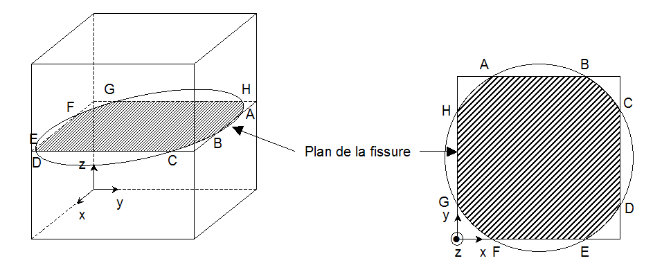
Figure 3.2.7-2 Case of a multiple crack background.

The vector. FONDMULT is an integer vector containing the indices of the starting and ending points of the various pieces of the crack bottom in the. FONDFISS. If NFONFI is the number of pieces of the crack bottom, then the vector. FONDMULT has a dimension of 2x NFONFI.

For example:

If FONDMULT = (1; 8; 9; 12)

So Piece No. 1 of the crack bottom: from point 1 to point 8 of the. FONDFISS

Piece no. 2 of the crack bottom: from point 9 to point 12 of the. FONDFISS

In 2D, each point on the crack bottom alone constitutes a background, the vector. However, FONDMULT was created. For example for 2 cracks, it will be equivalent to: FONDMULT = (1; 1; 2; 2)

The object is created provided that there is at least one point at the bottom of the crack.

3.2.8. . CARAFOND#

The vector. CARAFOND is a 2-dimensional real vector. It contains user settings concerning the crack background. The first component is the radius of enrichment of the elements and the second component is the number of layers of elements to be enriched.

So:

CARAFOND (1) = RAYON_ENRI if RAYON_ENRI is provided by the user,

0 otherwise.

CARAFOND (2) = NB_COUCHES if NB_COUCHES is provided by the user,

0 otherwise.

This data is the data provided by the user in the DEFI_FISS_XFEM command. They are stored because they are used again in the PROPA_FISS command to generate a propagated crack.

3.2.9. . LTNS#

The vector. LTNS is a string vector containing the two tables associated with the crack. These tables can be accessed using the RECU_TABLE command.

The first table named FOND_FISS contains the coordinates of the crack bottom points.

In 2D, it consists of the crack background number and the coordinates \(x\) and \(y\). So, the table display will be:

NUME_FOND COOR_X COOR_Y

In 3D, it describes each crack bottom. Thus, for each crack bottom i, the table will provide the curvilinear abscissa and the coordinates of the points at the bottom of crack i. The table display will be:

NUME_FOND NUME_PT ABS_CURV COOR_X COOR_Y COOR_Z

The second table named NB_FOND_FISS contains the number of crack bottoms.

The construction of these tables is based on the use of vectors. FONDFISS and. FONDMULT.

3.2.10. . LTNT#

The vector. LTNT is a string vector containing the names of the two tables associated with the crack to be supplied to the RECU_TABLE command. It’s FOND_FISS and NB_FOND_FISS.

3.2.11. . FOND. TAILLE_R#

This vector contains, for each of the background nodes, an estimate of the maximum size according to the direction of propagation, of the meshes that are connected to them. These sizes are ordered according to the order of the nodes given in the vector. FONDFISS.

We note \(\overrightarrow{{V}_{{P}_{i}}}\) the propagation vector from the local base to the background node Ni and \(\vec{{a}_{\mathit{ijk}}}\) the th edge of the th mesh to which the node Ni belongs.

For each node in the background Ni, the edges \(\vec{{a}_{\mathit{ijk}}}\) are projected onto the propagation direction vector \(\overrightarrow{{V}_{{P}_{i}}}\). The maximum size \({T}_{i}\) of the cells connected to Ni is the maximum value of the absolute values of its projections. In other words, the size \({T}_{i}\) is equal to

\({T}_{i}=\underset{\begin{array}{c}1\le j\le {\mathit{Nb}}_{\mathit{mailles},i}\\ 1\le k\le {\mathit{Nb}}_{\mathit{arêtes},j}\end{array}}{\mathit{max}}\left(∣\vec{{a}_{\mathit{ijk}}}\mathrm{.}\vec{{V}_{{P}_{i}}}∣\right)\),

where \({\mathit{Nb}}_{\mathit{mailles},i}\) is the number of meshes connected to the Ni node and \({\mathit{Nb}}_{\mathit{arêtes},j}\) is the number of edges of the jth mesh connected to the Ni node.

3.2.12. . NOFACPTFON#

'. NOFACPTFON ': S V I

This object contains the numbers of the vertex nodes (global mesh numbering) of the faces of the parent elements containing the crack bottom points.

Either:

V =. NOFACPTFON

NFON = number of points at the bottom of the crack

n = LONG (V) = 4x NFON

for i = 1, NFON:

V (4* (i-1) +1)	global number of the 1st vertex node of the face containing the bottom point number i
V (4* (i-1) +2)	global number of the 2nd vertex node of the face containing the bottom point number i
V (4* (i-1) +3)	global number of the 3rd vertex node of the face containing the bottom point number i
V (4*(i-1) +4)	global number of the 4th vertex node of the face containing the bottom point number si the face is quadrangular 0if the face is triangular

Notes:

For each point at the bottom of the crack, the face whose node numbers are stored in . NOFACPTFONn is not necessarily unique (for example the degenerate case of a bottom point coinciding with an edge or a node): it is the last face found by the routine intfacdans xptfon (phase of finding the points at the bottom of the crack in the operator DEFI_FISS_XFEM)

**The object* . NOFACPTFONest created only if the structure contains a crack background.

3.3. Enrichment objects#

3.3.1. . GROUP_MA_ENRI#

The vector. GROUP_MA_ENRI contains the list of mesh numbers in the area to be enriched.

3.3.2. . GROUP_NO_ENRI#

The vector. GROUP_NO_ENRI contains the list of node numbers in the zone to be enriched.

Note that this vector can be deduced from. GROUP_MA_ENRI.

Note:

These last two vectors are stored because we want to reuse in PROPA_FISS the information related to the GROUP_MA_ENRI keyword from DEFI_FISS_XFEM. And the only way to transmit the information is to store the numbers of the stitches and knots of the GROUP_MA_ENRI meshes.

3.3.3. . STNO#

The concept. STNO is a node field (CHAM_NO) with an integer component, corresponding to the status of the node in question.

If the node has its support completely cut by the crack, its status is 1.
If the node is in a zone « close » (this concept is defined according to a criterion defined by the user) to the crack bottom, its status is equal to 2.
If the node meets the two previous conditions, its status is set to 3.
In all other cases, the status is 0.

3.3.4. . STNOR#

The concept. STNOR is exactly the same field as. STNO but with real components. It can therefore be used for visualization with Salome for example.

3.3.5. . MAILFISS. HEAV#

The vector. MAILFISS. HEAV is an integer vector containing the list of numbers of Heaviside enriched cells (« RONDE » mesh).

3.3.6. . MAILFISS. CTIP#

The vector. MAILFISS. CTIP is an integer vector containing the list of numbers of enriched Crack-Tip cells (mesh « CARREE »).

3.3.7. . MAILFISS. HECT#

The vector. MAILFISS. HECT is an integer vector containing the list of numbers of enriched Heaviside-Crack-Tip cells (mesh « RONDE - CARREE »).

3.3.8. . MAILFISS. CONT#

The vector. MAILFISS. CONT is an integer vector containing the list of cell numbers on which contact is defined for the crack. These are the meshes:

- - Be strictly intersected by the crack (type 1 in fig.)
  - Either presenting an edge (in 2D) or a face (in 3D) confused with the crack, and located on the slave side (type 2 in fig.)
  - Or, in multi-cracking, meshes presenting Heaviside enrichment for the crack in question and which fall into one of the first two categories for another crack (type 3 in fig.).

In fact, to limit the introduction of new elements during the implementation of contact with multi-cracking, the number of contact degrees of freedom is always equal to the number of Heaviside degrees of freedom, even if it means then setting the superfluous contact degrees of freedom to 0. Hence the need to include meshes of this third type in the group of « in contact » meshes (but their degrees of freedom will be set to 0).

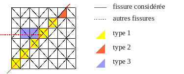
Figure 3.3.8-1 example of the group. MAILFISS. CONT of a crack.

3.3.9. . JONFISS#

The vector. JONFISS contains a list of the root cracks that the crack connects to. In particular, it is used in the MODI_MODELE_XFEM operator for multiple slicing and enrichment. This vector is created if the user makes use of the JONCTION keyword in DEFI_FISS_XFEM.

3.3.10. . JONCOEF#

The vector. JONCOEF is the same length as. JONFISS. It contains the list of coefficients to be associated with the normal crack level sets of. JONFISS to find the domain in which the plugged crack is defined. These coefficients are equal to \(+1\) or \(\mathrm{-}1\) and are calculated automatically. The branched crack is then defined in the zone where for all the mother cracks \(i\), the products JONCOEF (i) *lsn (JONFISS (i)) are negative.

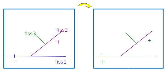
Figure 3.3.10-1 sign of the levels and the mother cracks on the left, sign obtained after multiplying by JONCOEF on the right, and definition of the plugged crack on the minus side.

In this way, it is ensured that the plugged crack is in the « minus » zone compared to the mother cracks. The figure shows an example of using. JONCOEFet of. JONFISSafin to define the crack 3. In this figure, the crack 3 is connected to the crack 2, which is itself connected to the crack 1,. JONFISSde crack 3 therefore contains cracks 1 and 2. The signs of the level sets of cracks 1 and 2 are given in the figure on the left: we deduce the values of JONCOEF \((\mathrm{-}\mathrm{1,1})\) as well as the distribution of the signs of \(\mathit{coef}(1)\mathrm{\times }\mathit{lsn}(1)\) and \(\mathit{coef}(2)\mathrm{\times }\mathit{lsn}(2)\) on the figure on the right. Fissure 3 is defined in the zone where the 2 signs are less.

In conclusion. JONFISSet. JONCOEFpermettent to define crack 3 with its usual normal and tangent level sets as well as the level and normal of the mother cracks, which can be accessed in an elementary way.

3.4. Propagation objects#

3.4.1. . PRO. RAYON_TORE#

Vector of real numbers with a length equal to 1.

In the case where this vector exists in the SD, the crack propagation was calculated using the location of the level sets update domain. The domain coincides with a 3D torus or a 2D circle built around the bottom of the crack. The radius of this torus or circle is stored in this object.

In the case where this vector does not exist in the SD, the whole model was used to calculate crack propagation.

3.4.2. . PRO. NOEUD_TORE#

A vector of booleans with a length equal to the number of nodes in the mesh on which the crack was defined or, in the case where a grid is associated with the crack, to the number of nodes in the grid.

In the case where this vector exists in the SD, the crack propagation was calculated using the location of the level sets update domain. For each node in the mesh (or grid), a value TRUE means that the node is within the domain used for the calculation. For example, if the value of the \(i\) th component of the vector is TRUE, the \(i\) th node of the mesh (or grid) is included in the domain; on the other hand, if the value of the \(i\) th component of the vector is FALSE, the \(i\) th node of the mesh (or grid) is outside the domain.

In the case where this vector does not exist in the SD, the whole model (or the whole grid) was used to calculate crack propagation.

3.4.3. . PRO. NOEUD_PROJ#

A vector of booleans with a length equal to the number of nodes in the mesh on which the crack was defined.

In the case where this vector exists in the SD, the crack propagation was calculated on the auxiliary grid associated with the crack and the calculated level sets were projected onto the mesh. For each node in the mesh, a value TRUE means that the node is within the projection domain. For example, if the value of the \(i\) th component of the vector is TRUE, the \(i\) th node of the mesh is included in the domain; on the other hand, if the value of the \(i\) th component of the vector is FALSE, the \(i\) th node of the mesh is outside the domain and the values of the level sets carried by this node have not been updated.

In the case where this vector does not exist in the SD, the crack propagation was calculated directly on the mesh.

3.4.4. . GRI. MAILLAGE#

K8 vector with a length equal to 1.

The name of the grid mesh associated with the crack. If this object does not exist, there is no grid associated with the crack.

3.4.5. . GRI. LTNO and. GRI. LNNO#

The concept. GRI. LTNO (resp.. GRI. LNNO) is a scalar node field (CHAM_NO) that contains for each node of the grid the real value of the level set tangent (resp. normal) to the crack. If this object does not exist, there is no grid associated with the crack.

3.4.6. . GRI. GRLTNO and. GRLNNO#

The concept. GRI. GRLTNO (resp.. GRI. GRLNNO) is a node field (CHAM_NO) with 3 real components. It contains for each node of the grid the values of the tangent level set gradient (resp. normal) in the 3 directions of space.

Let \(i\) be the \(i\) -th node in the grid,

V =. GRI. GRLTNO (i);

V (1)	Value of the next \(x\) gradient of the tangent level set, calculated at the \(i\) th node
V (2)	Value of the next \(y\) gradient of the tangent level set, calculated at the \(i\) th node
V (3)	Value of the gradient along z of the tangent level set, calculated at the \(i\) th node

In 2D, we only have 2 components following \(x\) and \(y\).

If this object does not exist, there is no grid associated with the crack.

3.4.7. . FONDFISG#

The vector. FONDFISG is a real vector containing the coordinates of the points of the crack bottom constructed on the auxiliary grid. The points are ordered according to the same method as that described in the document [R7.02.12] for creating the vector of the points of the crack background on the real mesh. FONDFISS, so that a curvilinear abscissa can be defined.

If NFON is the number of crack bottom points on the grid, then the length of the vector. FONDFISG is 4x NFON. For each point of the crack bottom on the grid, the first 3 components correspond to the 3 coordinates (in 3D) of the point, and the fourth component is its curvilinear abscissa.

This object is created only in 3D as part of crack propagation using the Upwind or Simplex methods as tools for updating level sets.

3.5. Contact objects#

These objects are created in sd_fiss_xfem by DEFI_CONTACT.

3.5.1. . BASCO#

The concept. BASCO is a node field (CHAM_NO) with 12 real components (in 2D and 3D). It contains the origin and vectors of the BASe COvariante of contact facets. For each node, the first three components are the coordinates of the contact point associated with that node, which corresponds to the origin of the covariant base. The next three components are the coordinates of the 1st vector in the base. The next three components are the coordinates of the 2nd vector in the base. The last three components are the coordinates of the 3rd vector in the base.

Let \(i\) be the \(i\) th node of the mesh,

V =. BASCO (i);

V (1)	Next coordinate \(x\) of the contact point associated with node \(i\)
V (2)	Next coordinate \(y\) of the contact point associated with node \(i\)
V (3)	Next coordinate \(z\) of the contact point associated with node \(i\)
V (4)	Next coordinate \(x\) of the 1st vector from the base to the point of contact associated with node \(i\)
V (5)	Next coordinate \(y\) of the 1st vector from the base to the point of contact associated with node \(i\)
V (6)	Next coordinate \(z\) of the 1st vector from the base to the point of contact associated with node \(i\)
V (7)	Next coordinate \(x\) of the 2nd vector from the base to the point of contact associated with node \(i\)
V (8)	Next coordinate \(y\) of the 2nd vector from the base to the point of contact associated with node \(i\)
V (9)	Next coordinate \(z\) of the 2nd vector from the base to the point of contact associated with node \(i\)
V (10)	Next coordinate \(x\) of the 3rd vector from the base to the point of contact associated with node \(i\)
V (11)	Next coordinate \(y\) of the 3rd vector from the base to the point of contact associated with node \(i\)
V (12)	Next coordinate \(z\) of the 3rd vector from the base to the point of contact associated with node \(i\)

In 2D, the components following \(z\) are zero.

3.5.2. . LISEQ (address JLIS1)#

It is the LISte of equal relationships (EQuality) between contact strangers.

Vector of integers of length NRELEQ *2 where NRELEQ is the number of equality relationships.

For each equality relationship, we store the numbers of the 2 nodes that are part of the equality:

Let IE be the \(i\) th relationship of equality,

ZI (JLIS1 -1+2* (IE-1) +1) is the number of the 1st node that is part of the tie.

ZI (JLIS1 -1+2* (IE-1) +2) is the number of the 2nd node that is part of the tie.

3.5.3. . LISEQ_LAGR (address JLISLA)#

This is the LISte of LAGRange issues associated with equal relationships (EQuality) between contact strangers. This list is built in the case of Multi-Heaviside meshes. It makes it possible to find the Lagrange ddl number to be associated with the number of a node in an equal relationship.

ZI (JLISLA -1+2* (IE-1) +1) is the Lagrange number to be associated with the 1st node of the equality relationship.

ZI (JLISLA -1+2* (IE-1) +2) is the Lagrange number to be associated with the 2nd node of the equality relationship.

For example, if we have to impose the relationship LAGS_C = LAG3_C between the nodes” N26 “and” N32 “for the th equality relationship, we will have:

ZI (JLIS1 -1+2* (IE-1) +1) = 26

ZI (JLIS1 -1+2* (IE-1) +2) = 32

ZI (JLISLA -1+2* (IE-1) +1) = 1

ZI (JLISLA -1+2* (IE-1) +2) = 3

3.5.4. . CNCTE (address JCNTES)#

These are groups of connected vital edges. For each local edge number in a mesh, which belongs to a group, we increment NCTE and we store:

ZI (JCNTES -1+4* (NCTE -1) +1) the number of the edge in the group,

ZI (JCNTES -1+4* (NCTE -1) +2) the group number,

ZI (JCNTES -1+4* (NCTE -1) +3) the mesh number,

ZI (JCNTES -1+4* (NCTE -1) +4) the local number of the edge in the mesh.