1. Reference problem#

1.1. Geometry#

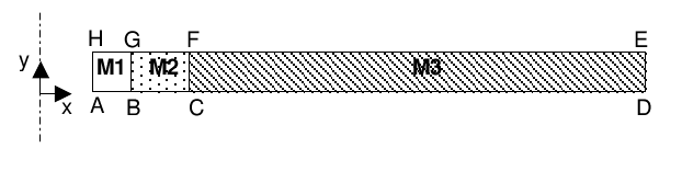
The domain is an axi-symmetric slice:

Coordinates of the points:

Point	\(X\)	\(Y\)
\(A\)	0.3075	0
\(B\)	0.3375	0
\(C\)	0.5375	0
\(D\)	200	0
\(E\)	200	1
\(F\)	0.5375	1
\(G\)	0.3375	1
\(H\)	0.3075	1

Area \(\mathrm{M1}\) represents the game and is made of the material \(\mathrm{MATJEU}\).

Zone \(\mathrm{M2}\) represents the damaged area and is made of material \(\mathrm{MATZE}\).

Zone \(\mathrm{M3}\) represents the clay in the field and is made of the material \(\mathrm{MATCOX}\).

1.2. Material properties#

Only the properties on which the solution depends are given here, knowing that the command file contains other material data that plays no role in solving the problem at hand.

\(\mathrm{MATJEU}\)
Liquid water	Density ( \({\mathrm{kg.m}}^{-3}\) ) Viscosity (\({\mathrm{kg.m}}^{-1}\mathrm{.}{s}^{-1}\)) Compressibility (\({\mathrm{Pa}}^{-1}\))	1000 10-3 0.5 10-9



Gaz	Density ( \({\mathrm{kg.m}}^{-3}\) ) Viscosity (\({\mathrm{kg.m}}^{-1}\mathrm{.}{s}^{-1}\))	2 10-3 1.8 10-5



Dissolved gas	Henry’s coefficient (\(\mathrm{Pa.}{\mathrm{mol}}^{-1}{m}^{3}\))	1870
Vapeur	Density (\({\mathrm{kg.m}}^{-3}\))	18 10-3
Homogenized parameters	Permeability \(K\) ( \({m}^{2}\) ) Porosity Fick gas (\({m}^{2}\mathrm{.}{s}^{-1}\)) Fick liquid (\({m}^{2}\mathrm{.}{s}^{-1}\)) Porosity	1.019 10-13 0.3 0.0015. (\(\mathrm{Smax}-S\)) 4.47 10-10. \(S\)




Van-Genuchten parameters	\(N\) \(\mathrm{Pr}\) (\(\mathrm{Mpa}\)) \(\mathrm{Sr}\) \(\mathrm{Smax}\)	1.064 4.91 10-3 0.08 0.999


Initial state	Capillary pressure (\(\mathrm{Mpa}\)) Gas pressure (\(\mathrm{Mpa}\))

\(\mathrm{MATZE}\)
Liquid water	Density ( \({\mathrm{kg.m}}^{-3}\) ) Viscosity (\({\mathrm{kg.m}}^{-1}\mathrm{.}{s}^{-1}\)) Compressibility (\({\mathrm{Pa}}^{-1}\))	1000 10-3 0.5 10-9



Gaz	Density ( \({\mathrm{kg.m}}^{-3}\) ) Viscosity (\({\mathrm{kg.m}}^{-1}\mathrm{.}{s}^{-1}\))	2 10-3 1.8 10-5



Dissolved gas	Henry’s coefficient (\(\mathrm{Pa.}{\mathrm{mol}}^{-1}{m}^{3}\))	1870
Vapeur	Density (\({\mathrm{kg.m}}^{-3}\))	18 10-3
Homogenized parameters	Permeability K ( \({m}^{2}\) ) Porosity Fick gas (\({m}^{2}\mathrm{.}{s}^{-1}\)) Fick liquid (\({m}^{2}\mathrm{.}{s}^{-1}\))	5.097 10-18 0.15 0.00075. (\(\mathrm{Smax}-S\)) 2.24 10-10.S



Van-Genuchten parameters	\(N\) \(\mathrm{Pr}\) (\(\mathrm{Mpa}\)) \(\mathrm{Sr}\) \(\mathrm{Smax}\)	1.5 4.91 0 0.999


Initial state	Capillary pressure (\(\mathrm{Mpa}\)) Gas pressure (\(\mathrm{Mpa}\))

\(\mathrm{MATCOX}\)
Liquid water	Density ( \({\mathrm{kg.m}}^{-3}\) ) Viscosity (\({\mathrm{kg.m}}^{-1}\mathrm{.}{s}^{-1}\)) Compressibility (\({\mathrm{Pa}}^{-1}\))	1000 10-3 0.5 10-9



Gaz	Density ( \({\mathrm{kg.m}}^{-3}\) ) Viscosity (\({\mathrm{kg.m}}^{-1}\mathrm{.}{s}^{-1}\))	2 10-3 1.8 10-5



Dissolved gas	Henry’s coefficient (\(\mathrm{Pa.}{\mathrm{mol}}^{-1}{m}^{3}\))	1870
Vapeur	Density (\({\mathrm{kg.m}}^{-3}\))	18 10-3
Homogenized parameters	Permeability \(K\) ( \(\mathrm{m2}\) ) Porosity Fick gas (\({m}^{2}\mathrm{.}{s}^{-1}\)) Fick liquid (\({m}^{2}\mathrm{.}{s}^{-1}\)) Porosity	5.097 10-21 0.15 0.00075. (Smax-S) 2.24 10-10.S




Van-Genuchten parameters	\(N\) \(\mathrm{Pr}\) (\(\mathrm{Mpa}\)) \(\mathrm{Sr}\) \(\mathrm{Smax}\)	1.49 14.7 0.01 0.999


Initial state	Capillary pressure (\(\mathrm{Mpa}\)) Gas pressure (\(\mathrm{Mpa}\))

The saturation and permeability curves follow the Mualem-Van-Genuchten model (HYDR_VGM). It is therefore necessary to define in the materials the parameters \(N\), \(\mathrm{Pr}\),, \(\mathrm{Sr}\), \(\mathrm{Smax}\).

It should be noted that these models are:

and

Relative permeability to water is expressed by integrating the prediction model proposed by Mualem (1976) into Van Genuchten’s capillarity model.

The permeability to gas is formulated in a similar way:

We recall that for \(S>\mathrm{Smax}\), these curves are interpolated by a polynomial of degree 2 \(\mathrm{C1}\) in \(\mathrm{Smax}\).

1.3. Boundary and initial conditions#

A hydrogen flow and a water flow are imposed on the left border (corrosion modeling):

\({\mathrm{Flux}}_{\mathrm{H20}}=-\mathrm{2,13}{.10}^{-10}\mathrm{kg}/{m}^{2}s\)

\({\mathrm{Flux}}_{\mathrm{H2}}=\mathrm{2,37}{.10}^{-11}\mathrm{kg}/{m}^{2}s\)

Initially, the initial capillary pressure is:

For game \(\mathrm{Pc}=\mathrm{5,18}\mathrm{Mpa}\)
For the damaged area and the Cox: \(1\mathrm{atm}\)

The gas pressure is initially \(1\mathrm{atm}\) everywhere.