2. Benchmark solution#
The total poroelastic stresses are: \(\sigma ={E}_{0}\varepsilon (u)-{\mathrm{bP}}_{\mathrm{lq}}\). Only the vertical component is present: \({\sigma }_{\mathrm{yy}}(y,t)={E}_{0}{u}_{y,y}(y,t)-{\mathrm{bP}}_{\mathrm{lq}}(y,t)\).
The poroelastic hydro-mechanical balance \(\mathrm{1D}\) is therefore written, in the absence of force of gravity, for \(t\ge 0\):
\(\{\begin{array}{c}{E}_{0}{u}_{y,\mathrm{yy}}(y,t)-{\mathrm{bP}}_{\mathrm{lq},y}(y,t)=0,\mathrm{équilibre}\mathrm{mécanique}\\ {\lambda }_{\mathrm{lq}}^{H}{P}_{\mathrm{lq},\mathrm{yy}}(y,t)-b{\dot{u}}_{y,y}(y,t)=0,\mathrm{équilibre}\mathrm{hydraulique}\end{array}\)
with the initial conditions: \({u}_{y}(y\mathrm{,0})=0\), \({P}_{\mathrm{lq}}(y\mathrm{,0})=0\) and the boundary conditions for \(t>0\): \({u}_{y}(\mathrm{0,}t)=0\), \({P}_{\mathrm{lq}}(\mathrm{0,}t)=0\), \({\sigma }_{\mathrm{yy}}(H,t)={F}_{0}\eta (t)={E}_{0}{u}_{y,y}(H,t)-{\mathrm{bP}}_{\mathrm{lq}}(H,t)\) where \(\eta (t)\) is the echelon function in \(t=0\) (Heaviside).
The mechanical balance directly gives the uniformity of the total stresses for \(t>0\) on \(∣\mathrm{0,}H∣\), hence: \({\sigma }_{\mathrm{yy}}(y,t)={F}_{0}={E}_{0}{u}_{y,y}(y,t)-{\mathrm{bP}}_{\mathrm{lq}}(y,t)\), or \({u}_{y,y}(y,t)=\frac{1}{{E}_{0}}({F}_{0}+{\mathrm{bP}}_{\mathrm{lq}}(y,t))\), for \(t>0\) on \(∣\mathrm{0,}H∣\).
Hydraulic balance then leads to:
\(\frac{{b}^{2}}{{E}_{0}}{\dot{P}}_{\mathrm{lq}}(y,t)-{\lambda }_{\mathrm{lq}}^{H}{P}_{\mathrm{lq},\mathrm{yy}}(y,t)=0\), for \(t>0\) out of \(∣\mathrm{0,}H∣\)
with \({P}_{\mathrm{lq}}(y\mathrm{,0})=-\frac{{F}_{0}}{b}\) on \(∣\mathrm{0,}H∣\) as initial conditions, and two boundary conditions \({P}_{\mathrm{lq}}(H,t)=0\) and \({P}_{\mathrm{lq},y}(\mathrm{0,}t)=0\) for \(t>0\), i.e. a thermal shock problem on \(∣\mathrm{0,}H∣\).
The consolidation coefficient \({c}_{\nu }={\lambda }_{\mathrm{lq}}^{H}{E}_{0}/{b}^{2}\) applies here: \({c}_{\nu }=\mathrm{0,1}{m}^{2}/s\). It controls the duration of the consolidation process.
This thus results in a characteristic time \({\tau }_{c}={H}^{2}/{c}_{\nu }\) (\(\mathrm{=}\mathrm{1000s}\) here) used to identify the time discretization step for the numerical integration method. At this value \({\tau }_{c}\), just over 90% of the consolidation has been achieved.
The solution is, cf. [2]:
\({P}_{\mathrm{lq}}(y,t)=\frac{-4{F}_{0}}{\pi b}\sum _{m=\mathrm{1,2}\mathrm{,3}\mathrm{..}}^{+\infty }\frac{{(-1)}^{m-1}}{\mathrm{2m}-1}{e}^{-{\lambda }_{\mathrm{lq}}^{H}{E}_{0}{\pi }^{2}{(\mathrm{2m}-1)}^{2}\frac{t}{({\mathrm{4b}}^{2}{H}^{2})}}\mathrm{.}\mathrm{cos}(\frac{\pi y(\mathrm{2m}-1)}{\mathrm{2H}})\)
and: \({u}_{y}(y,t)=\frac{{F}_{0}y}{{E}_{0}}+\frac{b}{{E}_{0}}\underset{0}{\overset{y}{\int }}{P}_{\mathrm{lq}}(\xi ,t)d\xi\)
That is: \({u}_{y}(y,t)=\frac{{F}_{0}y}{{E}_{0}}-\frac{8H{F}_{0}}{{\pi }^{2}{E}_{0}}\sum _{m=\mathrm{1,2}\mathrm{,3}\mathrm{..}}^{+\infty }\frac{{(-1)}^{m-1}}{{(\mathrm{2m}-1)}^{2}}{e}^{-{\lambda }_{\mathrm{lq}}^{H}{E}_{0}{\pi }^{2}{(\mathrm{2m}-1)}^{2}\frac{t}{({\mathrm{4b}}^{2}{H}^{2})}}\mathrm{.}\mathrm{sin}(\frac{\pi y(\mathrm{2m}-1)}{\mathrm{2H}})\)
The effective constraints (acting on the skeleton) are: \({\sigma }_{\mathrm{yy}}^{\mathrm{eff}}(y,t)={E}_{0}{u}_{y,y}(y,t)\) .For moments \(t\to \infty\), we get: \({P}_{\mathrm{lq}}(\mathrm{0,}\infty )=0\) and \({u}_{y}(H,\infty )=\frac{{F}_{0}H}{{{\rm E}}_{0}}\) (i.e. here \(-{10}^{-6}m\)).
2.1. Uncertainties about the solution#
The reference solution is analytical.
2.2. Influence of the choice of modeling#
In this paragraph, we want to draw attention to a numerical modeling difficulty associated with this type of test (Terzaghi column). In the following, we therefore discuss the influence of the modeling chosen and we rely in particular on calculations carried out with the Lagamine code (University of Liège) which has elements different from those of Code_Aster. For this reason, the test presented in this paragraph comes from an external study and is not quantitatively exactly the same as that studied in the rest of the document. It therefore does not give the same reference solutions. This paragraph is therefore a supplement given for information purposes.
At instant \(t=0\), the solution is discontinuous at the free surface \(y=H\):
\(\{\begin{array}{cc}\frac{{P}_{\mathit{lq}}(y\mathrm{,0})}{{F}_{0}}=1& \forall y<H\\ {P}_{\mathit{lq}}(H\mathrm{,0})=0& \end{array}\)
Because of this discontinuity, this test is a case study highlighting the phenomena of numerical oscillations in hydraulic pressure linked to the use of a mixed formulation by the finite element method. These oscillations generally occur in the vicinity of a draining wall, and are due to:
the violation of the inf-sup condition;
choosing a time step that is too small, violating the principle of maximum [:ref:`**R3.06.07**<**R3.06.07* >`];
The choice of the type of finite elements has a considerable influence on the solution obtained in the vicinity of the free surface, around \(t=0\). In Code_Aster, selective modelling (HMS) eliminates these oscillations (Figure 2.2-a), unlike classical modeling (HM).
However, obtaining the exact solution for hydraulic pressure \({P}_{\mathit{lq}}(y\mathrm{,0})\) by HMS modeling results in a greater approximation (compared to HM modeling, see the fine mesh case in Figure 2.2-b) for the solution in vertical displacement \({u}_{y}(y\mathrm{,0})\). This approximation is all the greater the coarser the mesh around the free surface.
Finally, we note that the displacement calculated by the Lagamine code (University of Liège) is perfectly accurate and independent of the fineness of the mesh, but with in return a very oscillating hydraulic pressure solution [:ref:` HT66-05-012-A < HT66-05-012-A >`]. This is due to the type of finite elements used by Lagamine which are different from ours since it is a P2P2 with a 9PG/9PG quadrature. This element does not satisfy the inf-sup condition and therefore cannot provide a correct hydraulic pressure solution.
2.3. Bibliographical references#
MEIROVITCH: Analytical methods in vibrations. McMillan Ed., 1967.
J.J. MARIGO, E. PLANCHAIS: Introduction to asymptotic methods. Application to linear thermal problems. Note EDF/DER/IMA/MMN HI-70/7563, 31/08/1992.
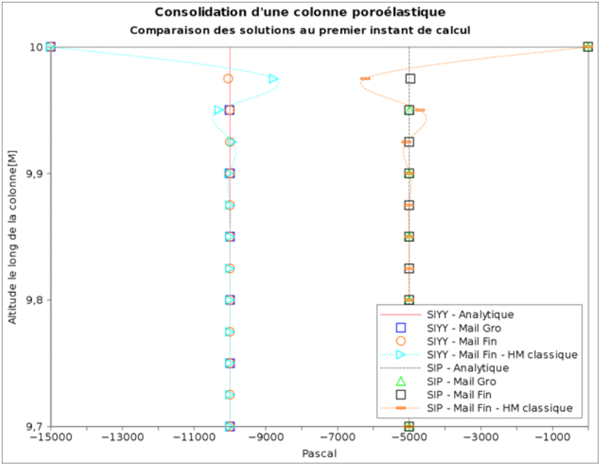
Figure 2.2-a: Comparison of the solutions in vertical effective constraints (SIYY) and in hydraulic pressure (SIP) obtained at the first calculation step in the vicinity of the free surface (following a vertical section) for different mesh sizes and for selective (HMS) and classical (HM) models in the case of « fine » meshing. Comparison with analytical solutions at \(t=0\).
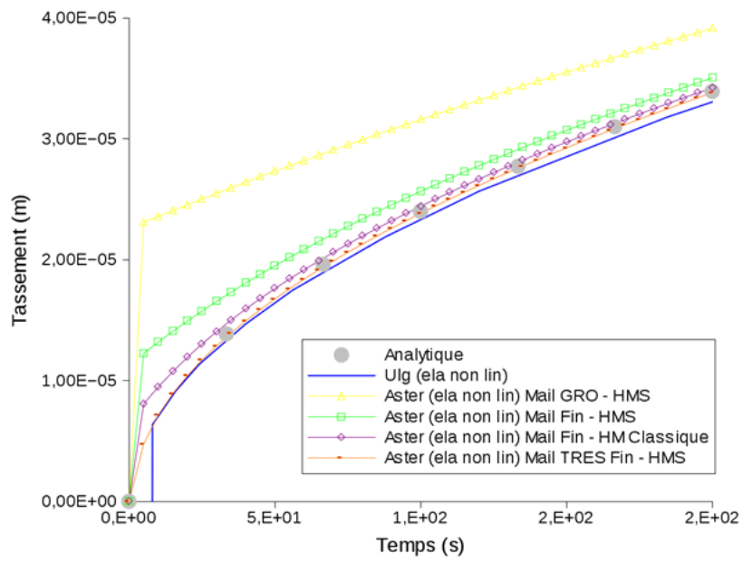
Figure 2.2-b: Comparison of the vertical displacement of the free surface as a function of time obtained for 3 different meshes and Lagamine for the « fine » mesh. Comparison of classical (HM) and selective (HMS) Code_Aster models for « fine » meshing. The analytical solution of the problem is also shown.