2. Modeling A#
2.1. Geometry and modeling#
The model has 4 discrete elements, 2 based on POI1 meshes and 2 on SEG2 meshes.
For each type of mesh, the first vector of the local coordinate system is oriented according to the vector \(X\) (global) for one cell and according to \(Y\) for the other. For POI1, we use the ORIENTATION keyword from AFFE_CARA_ELEM to impose this, for SEG2, this is imposed by geometry. This makes it possible to check that the REPERE keyword has been taken into account, which can take the values GLOBAL or LOCAL.
2.2. Settings#
The settings are as follows:
\(\mathrm{\omega }=2\mathrm{\pi }f\) with \(f=50\mathit{Hz}\)
\(K=(\mathrm{1,0,0})\), only longitudinal stiffness (according to the local \(x\) vector) is imposed
The orientation is chosen: (30,30,30) to validate unidirectional behavior in any frame of reference;
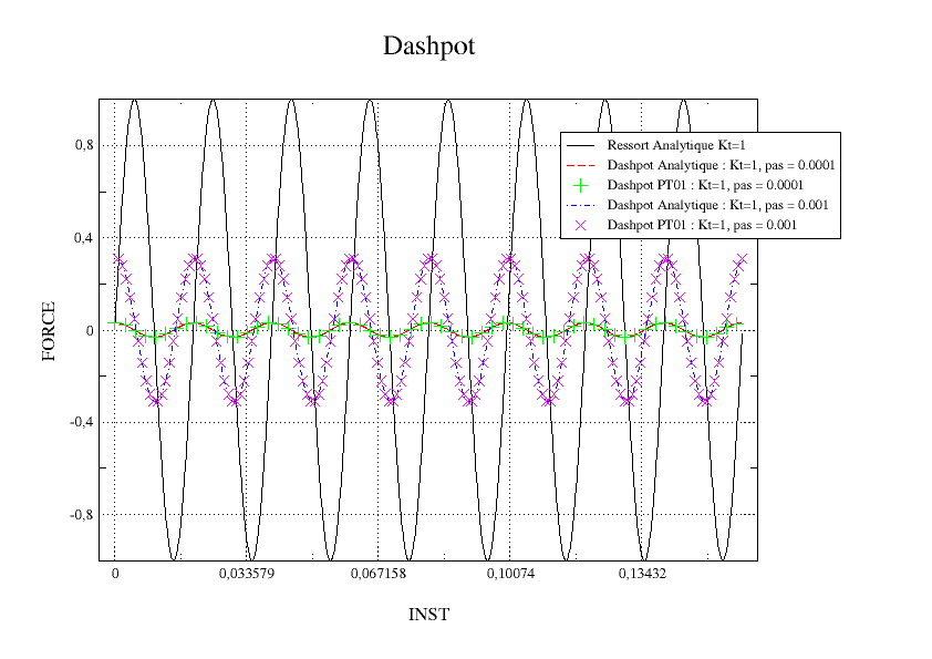
two values of \({\mathrm{\Delta }}_{t}\) are considered, a low value for the first calculation being \(1E-4\) inducing low displacement increments and therefore weak forces, and a larger value for the second calculation equal to \(1E-3\), inducing larger displacement increments and therefore greater forces.
2.3. Results#
For both calculations and for the 4 elements, we test the maximum of the differences between the analytical value and the calculated value at each moment of calculation. This maximum should be close to 0. For each calculation, this value is the same for all 4 elements. Moreover, as might be expected, the lower the time increment is, the closer you are to the analytical solution.
Identification |
Reference Type |
Reference Value |
Tolerance |
Calculation \({\mathrm{\Delta }}_{t}=1E-4\) |
ANALYTIQUE |
|
|
Calculation \({\mathrm{\Delta }}_{t}=1E-3\) |
ANALYTIQUE |
|
The following figure makes it possible to compare the calculated results with the analytical solutions for the two calculations performed.