1. Reference problem#
1.1. Geometry#
The geometry generated automatically in the macro command SIMU_POINT_MAT [U4.51.12] is unique and simple: it is a tetrahedron with side 1, at whose nodes linear relationships are applied to obtain a homogeneous state of stress and deformation.
1.2. Material properties#
Material characteristics are defined using the DEFI_MATERIAU command. The elastic characteristics are:
\(E=32000\mathrm{MPa}\) (except for D-modeling, see table below)
\(\nu =0.2\),
The other parameters describing the laws were chosen from Code_Aster test cases. The following table summarizes all the Code_Aster laws considered and the associated parameters:
Modeling |
Code_Aster laws of behavior |
parameters retained |
test used for the choice of parameters |
A |
BETON_RAG |
COMP_BETON = “ENDO_FLUA”,
|
Unrealistic values, for the purposes of the computer verification test. |
B |
BETON_UMLV
|
K_RS = 2.0E5 (MPa)
|
Parameters identical to test SSNV163A |
C |
BETON_BURGER
|
K_RS = 2.0E5 (MPa)
|
Parameters identical to test SSNV163D |
D |
ENDO_LOCA_EXP
|
E= 34129 (Mpa)
|
Parameters identical to test SSNV261A |
1.3. Boundary conditions and loads#
1.3.1. Characteristics of the loading path#
The proposed loading causes each component of the tensor to vary in a decoupled manner from the deformations in successive steps. A cyclic charge-discharge path is proposed by covering the states of traction and compression as well as an inversion of the signs of shear in order to test a wide range of values.
Schematically, it follows a course on 8 segments \(\mathrm{[}O\mathrm{-}A\mathrm{-}B\mathrm{-}C\mathrm{-}O\mathrm{-}C’\mathrm{-}B’\mathrm{-}A’\mathrm{-}O\mathrm{]}\) where the second part of the path \(\mathrm{[}O\mathrm{-}C’\mathrm{-}B’\mathrm{-}A’\mathrm{-}O\mathrm{]}\) is symmetric with respect to the origin of the first \(\mathrm{[}O\mathrm{-}A\mathrm{-}B\mathrm{-}C\mathrm{-}O\mathrm{]}\).
1.3.2. Application of requests#
We come back to the study of a material point (using the macro-command SIMU_POINT_MAT [U4.51.12]) by stressing an element in a homogeneous manner by imposing in \(\mathrm{3D}\), the 6 components of the deformation tensor:
\(\stackrel{ˉ}{\varepsilon }\mathrm{=}\left[\begin{array}{ccc}{\varepsilon }_{\mathit{xx}}& {\varepsilon }_{\mathit{xy}}& {\varepsilon }_{\mathit{xz}}\\ {\varepsilon }_{\mathit{xy}}& {\varepsilon }_{\mathit{yy}}& {\varepsilon }_{\mathit{yz}}\\ {\varepsilon }_{\mathit{xz}}& {\varepsilon }_{\mathit{yz}}& {\varepsilon }_{\mathit{zz}}\end{array}\right]\)
For a more general description, the imposed deformation tensor will be decomposed into a hydrostatic and deviatoric part on shear bases:
\(\stackrel{ˉ}{\varepsilon }\mathrm{=}\left[\begin{array}{ccc}{\varepsilon }_{\mathit{xx}}& {\varepsilon }_{\mathit{xy}}& {\varepsilon }_{\mathit{xz}}\\ {\varepsilon }_{\mathit{xy}}& {\varepsilon }_{\mathit{yy}}& {\varepsilon }_{\mathit{yz}}\\ {\varepsilon }_{\mathit{xz}}& {\varepsilon }_{\mathit{yz}}& {\varepsilon }_{\mathit{zz}}\end{array}\right]\mathrm{=}p\left[\begin{array}{ccc}1& 0& 0\\ 0& 1& 0\\ 0& 0& 1\end{array}\right]+{d}_{1}\left[\begin{array}{ccc}1& 0& 0\\ 0& \mathrm{-}1& 0\\ 0& 0& 1\end{array}\right]+{d}_{2}\left[\begin{array}{ccc}0& 0& 0\\ 0& 1& 0\\ 0& 0& \mathrm{-}1\end{array}\right]+\left[\begin{array}{ccc}0& {\varepsilon }_{\mathit{xy}}& {\varepsilon }_{\mathit{xz}}\\ {\varepsilon }_{\mathit{xy}}& 0& {\varepsilon }_{\mathit{yz}}\\ {\varepsilon }_{\mathit{xz}}& {\varepsilon }_{\mathit{yz}}& 0\end{array}\right]\) in \(\mathrm{3D}\)
1.3.3. Description of the imposed deformation path#
The path applied is described in the table below, the deformation values applied are calibrated with respect to the elastic modulus:
Segment number |
1 |
2 |
2 |
3 |
3 |
3 |
4 |
5 |
6 |
7 |
8 |
Segment |
\(O-A\) |
|
|
|
|
|
|
|
|||
\({\varepsilon }_{\mathit{xx}}\mathrm{\times }E\) |
787.5 |
1050 |
1050 |
350 |
350 |
0 |
-350 |
-1050 |
-787.5 |
0 |
|
\({\varepsilon }_{\mathit{yy}}\mathrm{\times }E\) |
525.0 |
-175 |
-175 |
-350 |
-350 |
175 |
525 |
0 |
|||
\({\varepsilon }_{\mathit{zz}}\mathrm{\times }E\) |
262.5 |
700 |
700 |
-525 |
-525 |
525 |
-700 |
-262.5 |
0 |
||
\({\varepsilon }_{\mathit{xy}}\mathrm{\times }E\mathrm{/}(1+\nu )\) |
700 |
350 |
350 |
1050 |
1050 |
-1050 |
-350 |
-700 |
0 |
||
\({\varepsilon }_{\mathit{xz}}\mathrm{\times }E\mathrm{/}(1+\nu )\) |
-350 |
350 |
350 |
700 |
700 |
0 |
-700 |
700 |
0 |
||
\({\varepsilon }_{\mathit{yz}}\mathrm{\times }E\mathrm{/}(1+\nu )\) |
0 |
700 |
-350 |
-350 |
0 |
350 |
-700 |
0 |
0 |
||
\(P\) |
525 |
525 |
525 |
-175 |
-175 |
-525 |
-525 |
0 |
|||
\(\mathrm{d1}\) |
262.5 |
525 |
525 |
525 |
0 |
-525 |
-525 |
-262.5 |
0 |
||
\(\mathrm{d2}\) |
262.5 |
-175 |
-175 |
350 |
350 |
0 |
-350 |
175 |
-262.5 |
0 |
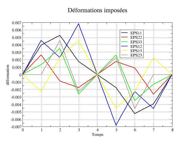
This path is illustrated by the following graph:
1.4. Initial conditions#
Zero stresses and deformations.