1. Reference problem#
1.1. Geometry#
The geometry (generated automatically in the macro command SIMU_POINT_MAT [U4.51.12]) is unique and simple: in 3D it is a tetrahedron on side 1, and in 2D it is a triangle on side 1, at whose nodes linear relationships are applied to obtain a state of homogeneous stress and deformation.
1.2. Material properties#
Material characteristics are defined for each behavior using the DEFI_MATERIAU command. The elastic and isotropic work-hardening characteristics selected are those of standard \(\mathrm{16MND5}\) steel:
\(E=200000\mathrm{MPa}\),
\(\nu =0.3\),
\({\sigma }_{y}=437\mathrm{MPa}\).
The other parameters describing the laws were chosen based on the ASTER test cases. The following two tables summarize all the laws of Code ASTER considered and the associated parameters:
Fashionable. |
Lois Code_Aster |
Parameters retained |
Criteria used for the choice of parameters |
A |
VMIS_ISOT_LINE
|
\(\mathrm{SY}=437\mathrm{MPa}\), \(\mathrm{DSY}=\mathrm{2024MPa}\) |
Material data \(\mathrm{16MND5}\) |
B |
VMIS_ISOT_TRAC
|
Traction curve at \(100°C\) from \(16\mathrm{MND5}\) |
Material data \(\mathrm{16MND5}\) |
C |
VMIS_CINE_LINE
|
\(\mathrm{SY}=437\mathrm{MPa}\), \(\mathrm{DSY}=\mathrm{2024MPa}\) |
Material data \(\mathrm{16MND5}\) |
D |
VMIS_ECMI_LINE
|
\(\mathrm{SY}=437\mathrm{MPa}\), \(\mathrm{DSY}=\mathrm{2024MPa}\) \({C}_{\mathrm{PRAG}}=1486.9\). |
Material data \(\mathrm{16MND5}\) |
E |
VMIS_ECMI_TRAC
|
Traction curve at \(100°C\) from \(16\mathrm{MND5}\) \({C}_{\mathrm{PRAG}}=1486.9\). |
Material data \(\mathrm{16MND5}\) |
F |
VMIS_CIN1_CHAB
|
\(\mathrm{SY}=437.0\);
|
work hardening: \(\mathrm{données16MND5}\) other parameters: ssnv101c |
G |
VMIS_CIN2_CHAB
|
\(\mathrm{SY}=437.0\);
|
|
H |
VMIS_ISOT_PUIS
|
\(\mathrm{SY}=437.0\);
|
|
J |
MOHR_COULOMB
|
\(E=\mathrm{619,3}\mathit{MPa}\)
|
Hostun sand |
K |
MohrCoulombAS
|
\(E=619.3\mathit{MPa}\)
|
Hostun sand |
L |
NLH_CSRM
|
YoungModulus=7.0E9
|
Fictional |
1.3. Boundary conditions and loads#
1.3.1. Characteristics of loading paths#
Two loading paths have been defined to deal with 3D and 2D plane cases. They are common to all laws of behavior. Each of them meets the following criteria:
an accumulated plastic deformation, \(p\), of 4 to 5% over the entire path,
a 1% increase in \(p\) during a portion of the trip,
This calibration was carried out on law VMIS_ISOT_LINE, then carried over to the other laws.
The proposed loading causes each component of the deformation tensor to vary in a decoupled manner by successive step. A cyclic load-discharge path is proposed by covering the states of traction and compression as well as an inversion of the signs of shear in order to test a wide range of values.
Schematically, it follows a course over 8 segments \([O-A-B-C-O-C’-B’-A’-O]\) where the second part of the path [O-C”-B”-A”-O] is symmetric with respect to the origin of the first \([O-A-B-C-O]\).
1.3.2. Application of requests#
We come back to the study of a material point (using the macro-command SIMU_POINT_MAT) by soliciting an element in a homogeneous manner by imposing:
in 3D, the 6 components of the deformation tensor:

in 2D the three components of the tensor:

For a more general description, the imposed deformation tensor will be decomposed into a hydrostatic and deviatoric part on shear bases:

in 2D,

In 3D
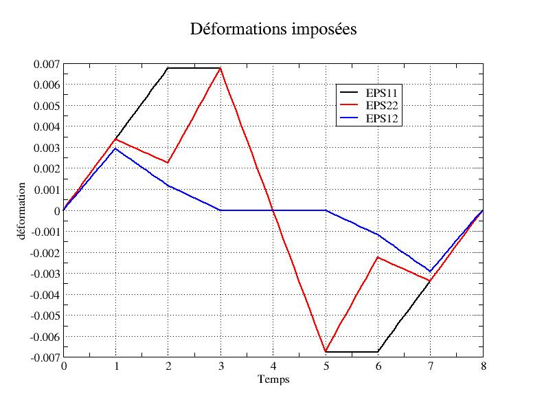
1.3.3. Description of the imposed deformation path in 2D#
The path applied is described in the table below, the deformation values are calibrated with respect to the elastic modulus:
Time |
1 |
2 |
3 |
3 |
3 |
4 |
5 |
6 |
7 |
8 |
Charging point |
\(A\) |
|
|
|
|
|
|
|
||
\({\varepsilon }_{\mathit{xx}}\mathrm{\times }E\) |
675 |
1350 |
1350 |
1350 |
0 |
-1350 |
-1350 |
-675 |
0 |
|
\({\varepsilon }_{\mathit{yy}}\mathrm{\times }E\) |
675 |
450 |
450 |
1350 |
1350 |
0 |
-1350 |
-450 |
-675 |
0 |
\({\varepsilon }_{\mathit{xy}}\mathrm{\times }E\mathrm{/}(1+\nu )\) |
450 |
180 |
180 |
0 |
0 |
0 |
-180 |
-450 |
0 |
|
\(P\) |
675 |
900 |
900 |
1350 |
-1350 |
-900 |
-675 |
0 |
||
\(D\) |
0 |
0 |
0 |
450 |
450 |
0 |
0 |
0 |
This path is illustrated by the following graph:
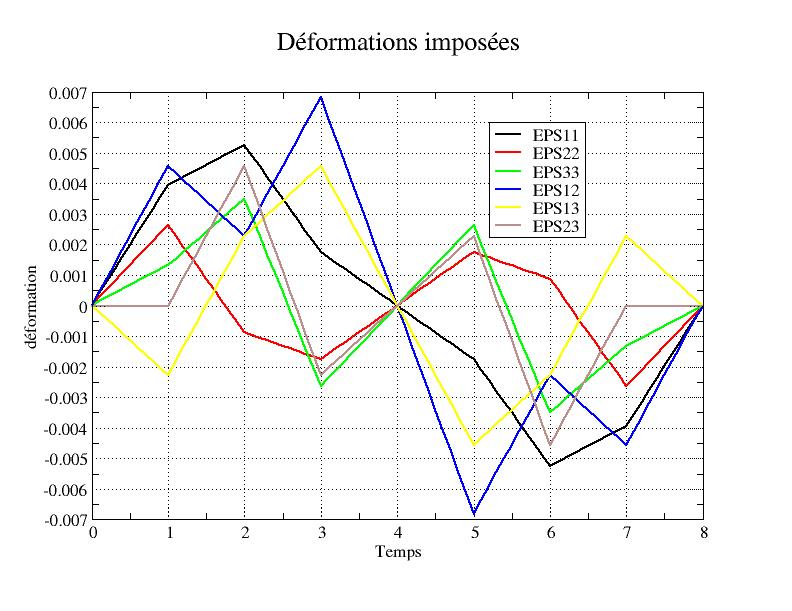
1.3.4. Description of the imposed deformation path in 3d#
The path applied is described in the table below, the deformation values applied are calibrated with respect to the elastic modulus:
Segment number |
1 |
2 |
2 |
3 |
3 |
3 |
4 |
5 |
6 |
7 |
8 |
Segment |
\(0-A\) |
|
|
|
|
|
|
|
|||
\({\varepsilon }_{\mathit{xx}}\mathrm{\times }E\) |
787.5 |
1050 |
1050 |
350 |
350 |
0 |
-350 |
-1050 |
-787.5 |
0 |
|
\({\varepsilon }_{\mathit{yy}}\mathrm{\times }E\) |
525.0 |
-175 |
-175 |
-350 |
-350 |
175 |
525 |
0 |
|||
\({\varepsilon }_{\mathit{zz}}\mathrm{\times }E\) |
262.5 |
700 |
700 |
-525 |
-525 |
525 |
-700 |
-262.5 |
0 |
||
\({\varepsilon }_{\mathit{xy}}\mathrm{\times }E\mathrm{/}(1+\nu )\) |
700 |
350 |
350 |
1050 |
1050 |
-1050 |
-350 |
-700 |
0 |
||
\({\varepsilon }_{\mathit{xz}}\mathrm{\times }E\mathrm{/}(1+\nu )\) |
-350 |
350 |
350 |
700 |
700 |
0 |
-700 |
700 |
0 |
||
\({\varepsilon }_{\mathit{yz}}\mathrm{\times }E\mathrm{/}(1+\nu )\) |
0 |
700 |
-350 |
-350 |
0 |
350 |
-700 |
0 |
0 |
||
\(P\) |
525 |
525 |
525 |
-175 |
-175 |
-525 |
-525 |
0 |
|||
\(\mathrm{d1}\) |
262.5 |
525 |
525 |
525 |
0 |
-525 |
-525 |
-262.5 |
0 |
||
\(\mathrm{d2}\) |
262.5 |
-175 |
-175 |
350 |
350 |
0 |
-350 |
175 |
-262.5 |
0 |
This path is illustrated by the following graph:
1.4. Initial conditions#
Zero stresses and deformations.