3. B modeling#
3.1. Characteristics of modeling#
The data is the same as modeling A.
3.2. Benchmark solution#
The equations are taken from [R7.01.26].
3.2.1. Chemical advancement#
Chemical advancement follows the following law:
\(\frac{\partial A}{\partial t}\phantom{\rule{2em}{0ex}}=\phantom{\rule{2em}{0ex}}{a}_{0}.\mathrm{exp}\left[\frac{{E}_{a}}{R}\left(\frac{1}{{T}_{\mathit{ref}}}-\frac{1}{T}\right)\right]\frac{{⟨{S}_{r}-{S}_{r}^{0}⟩}_{\text{+}}}{\left(1-{S}_{r}^{0}\right)}{⟨{S}_{r}-A⟩}_{\text{+}}\) [éq3.2.1-1]
This equation depends on temperature and drying. It can therefore be verified without knowing the state of deformation and stress of the sample.
3.2.2. Water pressure#
Capillary pressure is related to the degree of saturation, by the relationship:
\(\mathit{Pc}=-a.{S}_{r}.{({\mathit{Sr}}^{-b}-1)}^{1-1/b}\) [éq3.2.2-1]
This equation only depends on drying. It can therefore be verified without knowing the state of deformation and stress of the sample.
3.2.3. Gel pressure#
The effective freeze pressure follows the following law
\({P}_{\mathit{gel}}={b}_{g}.{M}_{g}{⟨A.{V}_{g}-{⟨{A}_{0}.{V}_{g}+{b}_{g}\mathit{tr}({\mathrm{\epsilon }}^{\mathit{total}})⟩}_{\text{+}}⟩}_{\text{+}}\) [éq3.2.3-1]
This equation depends on chemical progress and on the trace of deformation. It can therefore only be verified by knowing the state of deformation of the sample.
3.2.4. Mechanical condition of the sample#
To solve the preceding equations it is necessary to determine the constraints. The following equations govern the problem:
\({\mathrm{\epsilon }}^{\text{e}}=\frac{1+{\mathrm{\nu }}^{0}}{{E}^{0}}.{\mathrm{\sigma }}^{\text{e}}-\frac{{\mathrm{\nu }}^{0}}{{E}^{0}}\text{tr}({\mathrm{\sigma }}^{\text{e}}).\mathit{Id}\)
with:
\({\mathrm{\epsilon }}^{\text{total}}={\mathrm{\epsilon }}^{\text{e}}+{\mathrm{\epsilon }}^{\text{fluage}}+{\mathrm{\epsilon }}^{\text{vdt}}+{\mathrm{\epsilon }}^{\text{ther}}\)
\({\mathrm{\sigma }}^{\mathit{total}}={\mathrm{\sigma }}^{\text{e}}-{P}_{\mathit{gel}}.\mathit{Id}-{P}_{c}.\mathit{Id}\)
We are in the case where \({\mathrm{ϵ}}^{\mathit{total}}=0\) due to boundary conditions. The material parameters are chosen so that there is creep and that \({\mathrm{\epsilon }}^{\text{vdt}}=0\), \({\mathrm{\epsilon }}^{\text{ther}}=0\).
3.3. Tested sizes and results#
Chemical progress as well as capillary pressure do not depend on the state of stress or on the state of deformations. Their evolutions are identical to those of modeling A.
For chemical advancement, the corresponding internal variable is BR_AVCHI. The figure represents its evolution over time.
Instant |
Reference Value |
Precision |
|
10.00 |
4.981207357356948E-03 |
1.0E-03 |
|
40.00 |
5.361979299970E-01 |
1.0E-03 |
|
50.00 |
5.924644217241E-01 |
1.0E-03 |
|
80.00 |
5.938195769343E-01 |
1.0E-03 |
5.938195769343E-01 |
100.00 |
5.938216310035E-01 |
1.0E-03 |
|
110.00 |
5.9383380868086705E-01 |
1.0E-03 |
|
200.00 |
7.000000000002E-01 |
1.0E-03 |
For gel pressure, the corresponding internal variable is BR_PRGEL. The figure represents its evolution over time.
Instant |
Reference Value |
Precision |
40.00 |
2.101217954854E+06 |
1.0E-03 |
50.00 |
2.448598919982E+06 |
1.0E-03 |
80.00 |
2.460563938661E+06 |
1.0E-03 |
100.00 |
2.455008850947E+06 |
1.0E-03 |
110.00 |
2.455084251465E+06 |
1.0E-03 |
200.00 |
3.112433957654E+06 |
1.0E-03 |
For capillary pressure, the corresponding internal variable is BR_PRCAP. The figure represents its evolution over time.
Instant |
Reference Value |
Precision |
10.00 |
-2.810249099279E+06 |
1.0E-03 |
40.00 |
-2.529791246328E+06 |
1.0E-03 |
50.00 |
-2.400000000000E+06 |
1.0E-03 |
80.00 |
-2.861817604251E+06 |
1.0E-03 |
100.00 |
-2.142428528528563E+06 |
1.0E-03 |
110.00 |
-2.142428528528563E+06 |
1.0E-03 |
200.00 |
-2.142428528528563E+06 |
1.0E-03 |
For constraints, the names of the components in field SIEF_ELGA are SIXX, SIYY, SIZZ. Given the symmetry of the problem, the 3 constraints are identical. The figure shows the evolution of the stress over time.
Instant |
Reference Value |
Precision |
|
10.00 |
2.810249099279E+06 |
1.6E-02 |
|
40.00 |
4.285732914740E+05 |
1.2E-01 |
|
50.00 |
-4.8598919981998248E+04 |
1.1E+00 |
|
80.00 |
4.012536655895E+05 |
1.3E-01 |
4.012536655895E+05 |
100.00 |
-3.125803223844E+05 |
1.9E-01 |
|
110.00 |
-3.126557229023E+05 |
1.9E-01 |
|
200.00 |
-9.700054290914E+05 |
6.5E-02 |
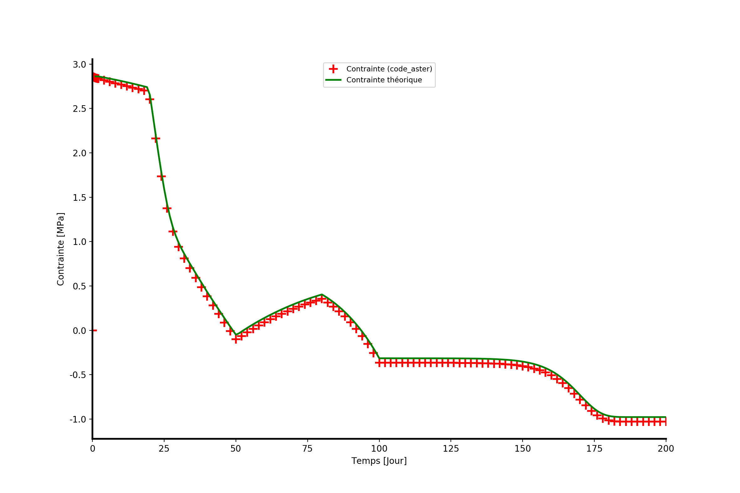
Figure 3.3-a : Constraints, comparison between the theoretical solution and that obtained by code_aster.