1. Reference problem#
1.1. Geometry#
According to the modeling \(\mathrm{2D}\) (plane deformation) or \(\mathrm{3D}\), we consider respectively a rectangle or a bar (see Figure 1.1-1).
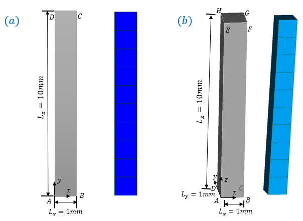
Figure 1.1-a : Geometry and Meshing of a rectangle (a) and a bar (b)
1.2. Material properties#
Elasticity:
\(E=190000\text{MPa}\) |
Young’s module |
\(\mathrm{\nu }=0.3\) |
Poisson’s ratio |
Work hardening curve:
\(R(\mathrm{\kappa })=488.36+57.13(1-\mathrm{exp}(-8613\mathrm{\kappa }))+238.73(1-\mathrm{exp}(-10.39\mathrm{\kappa }))\)
Ductile damage law GTN:
\({q}_{1}=1.5\) |
Model parameter GTN |
\({q}_{2}=1.07\) |
Model parameter GTN |
\({f}_{0}=0.0002i\) |
Initial porosity |
\({f}_{n}=0\) |
Germination Parameter |
\({f}_{c}=0.05\) |
Coalescence porosity |
\(\mathrm{\delta }=3\) |
Coalescent acceleration coefficient |
\(c=1N\) |
Non-local parameter |
\(r=5000\mathit{MPa}\) |
Lagrange penalty parameter |
Norton parameters in the viscoplastic case (C modeling):
\(n=14\) |
Exhibitor of Norton’s Law |
\(K=150\mathit{MPa}\mathrm{.}{s}^{1/14}\) |
Norton’s law coefficient |
In particular, the distribution of the initial porosity is not homogeneous. It increases with altitude: \({f}_{0}=0.0002i\) where \(i\) refers to the i-th element layer and \(1\le i\le 10\).
In DEFI_MATERIAU, the following information should be filled in:
ELAS |
ECRO_ NL |
**** NL |
GTN |
NON_LOCAL |
NORTON |
E = 190000 |
R0= 488.361 |
Q1 = 1.5 |
C_ GRAD_VARI = 1 |
N = 14 |
|
NU = 0.3 |
R1 = 57.133 |
Q2 = 1.07 |
|
K = 150 |
|
GAMMA_1 = 8613 |
|
||||
R2 = 238.731 |
|
||||
GAMMA_2 =10.386 |
|
1.3. Boundary conditions and loads#
For modeling \(2D\) (axisymmetric), the displacements along the \(X\) axis of all the nodes are controlled: \({u}_{x}=1.22x\), the displacements along the \(Y\) axis of the nodes of the same altitude remain uniform, the node \(A\) is blocked along the \(Y\) axis (see Figure 1.1-1 (a) for geometry).
For modeling \(3D\), the movements along the \(X\) axis and the \(Y\) movements of all the nodes are controlled: \({u}_{x}=1.22x\) and \({u}_{y}=1.22y\), the movements along the \(Z\) axis of the nodes of the same altitude remain uniform, the node \(A\) is blocked according to \(Z\). (see Figure 1.1-1 (b) for geometry).
Boundary conditions and loads are imposed this way so that the problem in \(2D\) and the problem in \(3D\) are the same.
The loading is applied at a constant speed for 1000 s. Time steps of 1 s each are imposed.